Concepts and Classes

Tutorial: Data access - Storage, View, Container

Note

This tutorial was generated from the python source [ptypy_root]/tutorial/ptypyclasses.py using ptypy/doc/script2rst.py. You are encouraged to modify the parameters and rerun the tutorial with:

$ python [ptypy_root]/tutorial/ptypyclasses.py

This tutorial explains how PtyPy accesses data / memory. The data access is governed by three classes: Container, Storage, and View

First a short reminder from the classes Module about the classes this tutorial covers.

Container class
    A high-level container that keeps track of sub-containers (Storage)
    and Views onto them. A container can copy itself to produce a buffer
    needed for calculations. Some basic Mathematical operations are
    implemented at this level as in-place operations.
    In general, operations on arrays should be done using the Views, which
    simply return numpy arrays.


Storage class
    The sub-container, wrapping a numpy array buffer. A Storage defines a
    system of coordinate (for now only a scaled translation of the pixel
    coordinates, but more complicated affine transformation could be
    implemented if needed). The sub-class DynamicStorage can adapt the size
    of its buffer (cropping and/or padding) depending on the Views.

View class
    A low-weight class that contains all information to access a 2D piece
    of a Storage within a Container. The basic idea is that the View
    access is controlled by a physical position and its frame, such that
    one is not bothered by memory/array addresses when accessing data.

Import some modules

>>> import matplotlib as mpl
>>> import numpy as np
>>> import ptypy
>>> from ptypy import utils as u
>>> from ptypy.core import View, Container, Storage, Base
>>> plt = mpl.pyplot

A single Storage in one Container

The governing object is a Container instance, which we need to construct as first object. It does not need much for an input but the data type.

>>> C1 = Container(data_type='real')

This class itself holds nothing at first. In order to store data in C1 we have to add a Storage to that container.

>>> S1 = C1.new_storage(shape=(1, 7, 7))

Similarly we can contruct the Storage from a data buffer. S1=C1.new_storage(data=np.ones((1,7,7))) would have also worked.

All of PtyPy’s special classes carry a uniue ID, which is needed to communicate these classes across nodes and for saving and loading.

As we haven’t specified an ID the Container class picks one for S1 In this case that will be S0000 where the S refers to the class type.

>>> print(S1.ID)
S0000

Let’s have a look at what kind of data Storage holds.

>>> print(S1.formatted_report()[0])
(C)ontnr : Memory : Shape            : Pixel size      : Dimensions      : Views
(S)torgs : (MB)   : (Pixel)          : (meters)        : (meters)        : act.
--------------------------------------------------------------------------------
S0000    :    0.0 :        1 * 7 * 7 :       1.0*1.0e0 :       7.0*7.0e0 :     0

Apart from the ID on the left we discover a few other entries, for example the quantity psize which refers to the physical pixel size for the last two dimensions of the stored data.

>>> print(S1.psize)
[1. 1.]

Many attributes of a Storage are in fact properties. Changing their value may have an impact on other methods or attributes of the class. For example, one convenient method is Storage.grids() that creates coordinate grids for the last two dimensions (see also ptypy.utils.array_utils.grids())

>>> y, x = S1.grids()
>>> print(y)
[[[-3. -3. -3. -3. -3. -3. -3.]
  [-2. -2. -2. -2. -2. -2. -2.]
  [-1. -1. -1. -1. -1. -1. -1.]
  [ 0.  0.  0.  0.  0.  0.  0.]
  [ 1.  1.  1.  1.  1.  1.  1.]
  [ 2.  2.  2.  2.  2.  2.  2.]
  [ 3.  3.  3.  3.  3.  3.  3.]]]

>>> print(x)
[[[-3. -2. -1.  0.  1.  2.  3.]
  [-3. -2. -1.  0.  1.  2.  3.]
  [-3. -2. -1.  0.  1.  2.  3.]
  [-3. -2. -1.  0.  1.  2.  3.]
  [-3. -2. -1.  0.  1.  2.  3.]
  [-3. -2. -1.  0.  1.  2.  3.]
  [-3. -2. -1.  0.  1.  2.  3.]]]

which are coordinate grids for vertical and horizontal axes respectively. We note that these coordinates have their center at

>>> print(S1.center)
[3 3]

Now we change a few properties. For example,

>>> S1.center = (2, 2)
>>> S1.psize = 0.1
>>> g = S1.grids()
>>> print(g[0])
[[[-0.2 -0.2 -0.2 -0.2 -0.2 -0.2 -0.2]
  [-0.1 -0.1 -0.1 -0.1 -0.1 -0.1 -0.1]
  [ 0.   0.   0.   0.   0.   0.   0. ]
  [ 0.1  0.1  0.1  0.1  0.1  0.1  0.1]
  [ 0.2  0.2  0.2  0.2  0.2  0.2  0.2]
  [ 0.3  0.3  0.3  0.3  0.3  0.3  0.3]
  [ 0.4  0.4  0.4  0.4  0.4  0.4  0.4]]]

>>> print(g[1])
[[[-0.2 -0.1  0.   0.1  0.2  0.3  0.4]
  [-0.2 -0.1  0.   0.1  0.2  0.3  0.4]
  [-0.2 -0.1  0.   0.1  0.2  0.3  0.4]
  [-0.2 -0.1  0.   0.1  0.2  0.3  0.4]
  [-0.2 -0.1  0.   0.1  0.2  0.3  0.4]
  [-0.2 -0.1  0.   0.1  0.2  0.3  0.4]
  [-0.2 -0.1  0.   0.1  0.2  0.3  0.4]]]

We observe that the center has in fact moved one pixel up and one left. The center() property uses pixel units. If we want to use a physical quantity to shift the center, we may instead set the top left pixel to a new value, which shifts the center to a new position.

>>> S1.origin -= 0.12
>>> y, x = S1.grids()
>>> print(y)
[[[-0.32 -0.32 -0.32 -0.32 -0.32 -0.32 -0.32]
  [-0.22 -0.22 -0.22 -0.22 -0.22 -0.22 -0.22]
  [-0.12 -0.12 -0.12 -0.12 -0.12 -0.12 -0.12]
  [-0.02 -0.02 -0.02 -0.02 -0.02 -0.02 -0.02]
  [ 0.08  0.08  0.08  0.08  0.08  0.08  0.08]
  [ 0.18  0.18  0.18  0.18  0.18  0.18  0.18]
  [ 0.28  0.28  0.28  0.28  0.28  0.28  0.28]]]

>>> print(x)
[[[-0.32 -0.22 -0.12 -0.02  0.08  0.18  0.28]
  [-0.32 -0.22 -0.12 -0.02  0.08  0.18  0.28]
  [-0.32 -0.22 -0.12 -0.02  0.08  0.18  0.28]
  [-0.32 -0.22 -0.12 -0.02  0.08  0.18  0.28]
  [-0.32 -0.22 -0.12 -0.02  0.08  0.18  0.28]
  [-0.32 -0.22 -0.12 -0.02  0.08  0.18  0.28]
  [-0.32 -0.22 -0.12 -0.02  0.08  0.18  0.28]]]

>>> print(S1.center)
[3.2 3.2]

Up until now our actual data numpy array located at S1.data is still filled with ones, i.e. flat. We can use Storage.fill to fill that container with an array.

>>> S1.fill(x+y)
>>> print(S1.data)
[[[-0.64 -0.54 -0.44 -0.34 -0.24 -0.14 -0.04]
  [-0.54 -0.44 -0.34 -0.24 -0.14 -0.04  0.06]
  [-0.44 -0.34 -0.24 -0.14 -0.04  0.06  0.16]
  [-0.34 -0.24 -0.14 -0.04  0.06  0.16  0.26]
  [-0.24 -0.14 -0.04  0.06  0.16  0.26  0.36]
  [-0.14 -0.04  0.06  0.16  0.26  0.36  0.46]
  [-0.04  0.06  0.16  0.26  0.36  0.46  0.56]]]

We can have visual check on the data using plot_storage()

>>> fig = u.plot_storage(S1, 0)

See Fig. 2 for the plotted image.

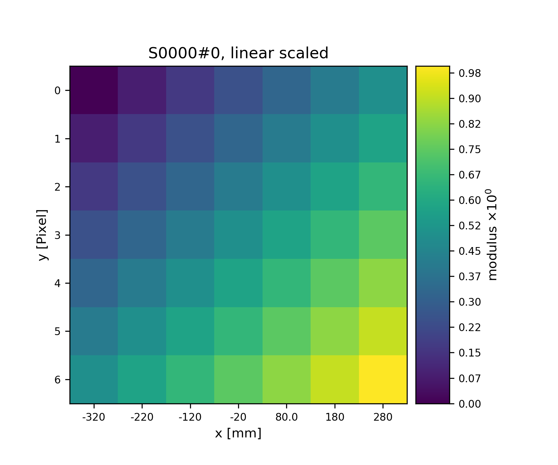
Fig. 2 A plot of the data stored in S1

Adding Views as a way to access data

Besides being able to access the data directly through its attribute and the corresponding numpy syntax, ptypy offers acces through a View instance. The View invocation is a bit more complex.

>>> from ptypy.core.classes import DEFAULT_ACCESSRULE
>>> ar = DEFAULT_ACCESSRULE.copy()
>>> print(ar)
* id3V1AJ3O73G           : ptypy.utils.parameters.Param(6)
  * storageID            : None
  * shape                : None
  * coord                : None
  * psize                : 1.0
  * layer                : 0
  * active               : True

Let’s say we want a 4x4 view on Storage S1 around the origin. We set

>>> ar.shape = (4, 4)  # ar.shape = 4 would have been also valid.
>>> ar.coord = 0.      # ar.coord = (0.,0.) would have been accepted, too.
>>> ar.storageID = S1.ID
>>> ar.psize = None

Now we can construct the View. Upon construction, the View will access information from Storage S1 to initialize other attributes for access and geometry.

>>> V1 = View(C1, ID=None, accessrule=ar)

We see that a number of the accessrule items appear in the View now.

>>> print(V1.shape)
[4 4]

>>> print(V1.coord)
[0. 0.]

>>> print(V1.storageID)
S0000

A few others were set by the automatic update of Storage S1.

>>> print(V1.psize)
[0.1 0.1]

>>> print(V1.storage)
          S0000 :    0.00 MB :: data=(1, 7, 7) @float64 psize=[0.1 0.1] center=[3.2 3.2]

The update also set new attributes of the View which all start with a lower d and are locally cached information about data access.

>>> print(V1.dlayer, V1.dlow, V1.dhigh)
0 [1 1] [5 5]

Finally, we can retrieve the data subset by applying the View to the storage.

>>> data = S1[V1]
>>> print(data)
[[-0.44 -0.34 -0.24 -0.14]
 [-0.34 -0.24 -0.14 -0.04]
 [-0.24 -0.14 -0.04  0.06]
 [-0.14 -0.04  0.06  0.16]]

It does not matter if we apply the View to Storage S1 or the container C1, or use the View internal View.data() property.

>>> print(np.allclose(data, C1[V1]))
True

>>> print(np.allclose(data, V1.data))
True

The first access yielded a similar result because the storageID S0000 is in C1 and the second acces method worked because it uses the View’s storage attribute.

>>> print(V1.storage is S1)
True

>>> print(V1.storageID in C1.S.keys())
True

We observe that the coordinate [0.0,0.0] is not part of the grid in S1 anymore. Consequently, the View was put as close to [0.0,0.0] as possible. The coordinate in data space that the View would have as center is the attribute pcoord() while dcoord() is the closest data coordinate. The difference is held by sp() such that a subpixel correction may be applied if needed (future release)

>>> print(V1.dcoord, V1.pcoord, V1.sp)
[3 3] [3.2 3.2] [0.2 0.2]

Note

Please note that we cannot guarantee any API stability for other attributes / properties besides .data, .shape and .coord

If we set the coordinate to some other value in the grid, we can eliminate the subpixel misfit. By changing the .coord property, we need to update the View manually, as the View-Storage interaction is non-automatic apart from the moment the View is constructed - a measure to prevent unwanted feedback loops.

>>> V1.coord = (0.08, 0.08)
>>> S1.update_views(V1)
>>> print(V1.dcoord, V1.pcoord, V1.sp)
[4 4] [4. 4.] [0. 0.]

We observe that the high range limit of the View is close to the border of the data buffer.

>>> print(V1.dhigh)
[6 6]

What happens if we push the coordinate further?

>>> V1.coord = (0.28, 0.28)
>>> S1.update_views(V1)
>>> print(V1.dhigh)
[8 8]

Now the higher range limit of the View is off bounds for sure. Applying this View to the Storage may lead to undesired behavior, i.e. array concatenation or data access errors.

>>> print(S1[V1])
[[0.16 0.26 0.36]
 [0.26 0.36 0.46]
 [0.36 0.46 0.56]]

>>> print(S1[V1].shape, V1.shape)
(3, 3) [4 4]

One important feature of the Storage class is that it can detect all out-of-bounds accesses and reformat the data buffer accordingly. A simple call to Storage.reformat() should do.

>>> print(S1.shape)
(1, 7, 7)

>>> mn = S1[V1].mean()
>>> S1.fill_value = mn
>>> S1.reformat()
>>> print(S1.shape)
(1, 4, 4)

Oh no, the Storage data buffer has shrunk! But don’t worry, that is intended behavior. A call to .reformat() crops and pads the data buffer around all active Views. We would need to set S1.padonly = True if we wanted to avoid that the data buffer is cropped. We leave this as an exercise for now. Instead, we add a new View at a different location to verify that the buffer will adapt to reach both Views.

>>> ar2 = ar.copy()
>>> ar2.coord = (-0.82, -0.82)
>>> V2 = View(C1, ID=None, accessrule=ar2)
>>> S1.fill_value = 0.
>>> S1.reformat()
>>> print(S1.shape)
(1, 15, 15)

Ok, we note that the buffer has grown in size. Now, we give the new View some copied values of the other view to make the View appear in a plot.

>>> V2.data = V1.data.copy()
>>> fig = u.plot_storage(S1, 2)

See Fig. 3 for the plotted image.

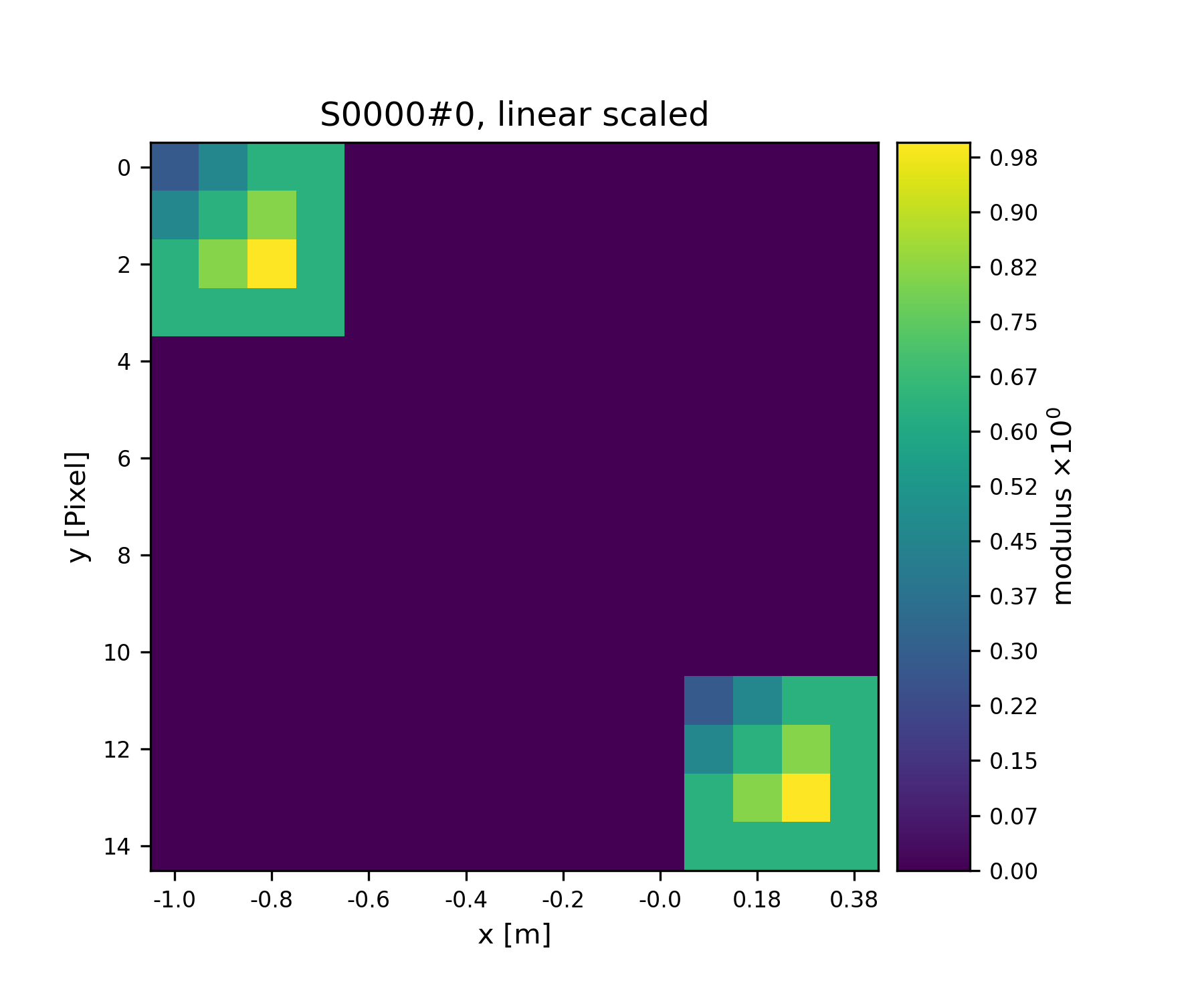
Fig. 3 Storage with 4x4 views of the same content.

We observe that the data buffer spans both views. Now let us add more and more Views!

>>> for i in range(1, 11):
>>>     ar2 = ar.copy()
>>>     ar2.coord = (-0.82+i*0.1, -0.82+i*0.1)
>>>     View(C1, ID=None, accessrule=ar2)
>>>

A handy method of the Storage class is to determine the coverage, which maps, for every pixel of the storage, the number of views having access to this pixel.

>>> S1.data[:] = S1.get_view_coverage()
>>> fig = u.plot_storage(S1, 3)

See Fig. 4 for the plotted image.

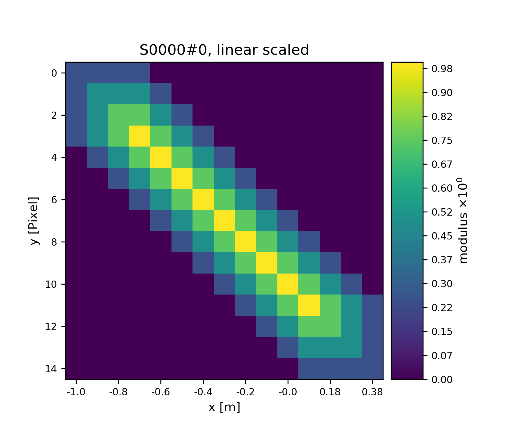
Fig. 4 View coverage of data buffer of S1.

Another handy feature of the View class is that it automatically creates a Storage instance to a storageID if that ID does not already exist.

>>> ar = DEFAULT_ACCESSRULE.copy()
>>> ar.shape = 200
>>> ar.coord = 0.
>>> ar.storageID = 'S100'
>>> ar.psize = 1.0
>>> V3=View(C1, ID=None, accessrule=ar)

Finally we have a look at the mischief we managed so far.

>>> print(C1.formatted_report())
(C)ontnr : Memory : Shape            : Pixel size      : Dimensions      : Views
(S)torgs : (MB)   : (Pixel)          : (meters)        : (meters)        : act.
--------------------------------------------------------------------------------
None     :    0.3 : float64
S0000    :    0.0 :      1 * 15 * 15 :      1.0*1.0e-1 :       1.5*1.5e0 :    12
S100     :    0.3 :    1 * 200 * 200 :       1.0*1.0e0 :       2.0*2.0e2 :     1

Tutorial: Modeling the experiment - Pod, Geometry

Note

This tutorial was generated from the python source [ptypy_root]/tutorial/simupod.py using ptypy/doc/script2rst.py. You are encouraged to modify the parameters and rerun the tutorial with:

$ python [ptypy_root]/tutorial/simupod.py

In the Tutorial: Data access - Storage, View, Container we have learned to deal with the basic storage-and-access classes on small toy arrays.

In this tutorial we will learn how to create POD and Geo instances to imitate a ptychography experiment and to use larger arrays.

We would like to point out that the “data” created her is not actual data. There is neither light or other wave-like particle involved, nor actual diffraction. You will also not find an actual movement of motors or stages, nor is there an actual detector. Everything should be understood as a test for this software. The selected physical quantities only simulate an experimental setup.

We start again with importing some modules.

>>> import matplotlib as mpl
>>> import numpy as np
>>> import ptypy
>>> from ptypy import utils as u
>>> from ptypy.core import View, Container, Storage, Base, POD
>>> plt = mpl.pyplot
>>> import sys
>>> scriptname = sys.argv[0].split('.')[0]

We create a managing top-level class instance. We will not use the the Ptycho class for now, as its rich set of methods may be a bit overwhelming to start with. Instead we start of a plain Base instance.

As the Base class is slotted starting with version 0.3.0, we can’t attach attributes after initialisation as we could with a normal python class. To reenable ths feature we have to subclasse once.

>>> class Base2(Base):
>>>     pass
>>>

>>> P = Base2()

Now we can start attaching attributes

>>> P.CType = np.complex128
>>> P.FType = np.float64

Set experimental setup geometry and create propagator

Here, we accept a little help from the Geo class to provide a propagator and pixel sizes for sample and detector space.

>>> from ptypy.core import geometry
>>> g = u.Param()
>>> g.energy = None  # u.keV2m(1.0)/6.32e-7
>>> g.lam = 5.32e-7
>>> g.distance = 15e-2
>>> g.psize = 24e-6
>>> g.shape = 256
>>> g.propagation = "farfield"
>>> G = geometry.Geo(owner=P, pars=g)

The Geo instance G has done a lot already at this moment. For example, we find forward and backward propagators at G.propagator.fw and G.propagator.bw. It has also calculated the appropriate pixel size in the sample plane (aka resolution),

>>> print(G.resolution)
[1.29882812e-05 1.29882812e-05]

which sets the shifting frame to be of the following size:

>>> fsize = G.shape * G.resolution
>>> print("%.2fx%.2fmm" % tuple(fsize*1e3))
3.32x3.32mm

Create probing illumination

Next, we need to create a probing illumination. We start with a suited container that we call probe

>>> P.probe = Container(P, 'Cprobe', data_type='complex')

For convenience, there is a test probing illumination in PtyPy’s resources.

>>> from ptypy.resources import moon_pr
>>> moon_probe = -moon_pr(G.shape)

As of version 0.3.0 the Storage classes are no longer limited to 3d arrays. This means, however, that the shape is better explicitly specified upon creation to align the coordinate system.

>>> pr_shape = (1,)+ tuple(G.shape)
>>> pr = P.probe.new_storage(shape=pr_shape, psize=G.resolution)

Probe is loaded through the fill() method.

>>> pr.fill(moon_probe)
>>> fig = u.plot_storage(pr, 0)

See Fig. 5 for the plotted image.

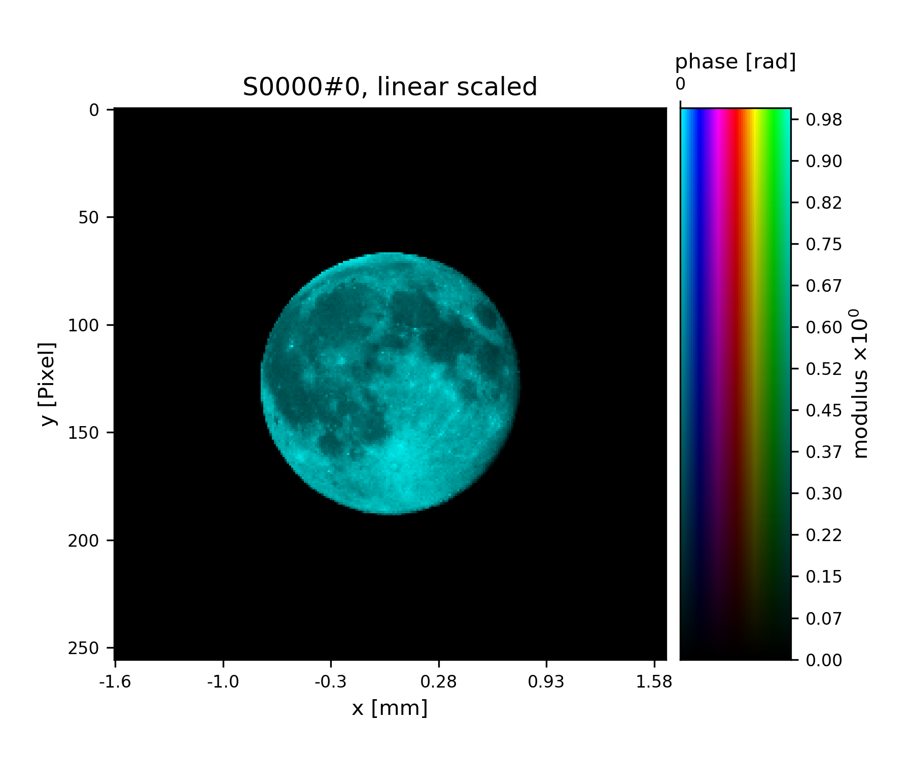
Fig. 5 Ptypy’s default testing illumination, an image of the moon.

Of course, we could have also used the coordinate grids from the propagator to model a probe,

>>> y, x = G.propagator.grids_sam
>>> apert = u.smooth_step(fsize[0]/5-np.sqrt(x**2+y**2), 1e-6)
>>> pr2 = P.probe.new_storage(shape=pr_shape, psize=G.resolution)
>>> pr2.fill(apert)
>>> fig = u.plot_storage(pr2, 1, channel='c')

See Fig. 6 for the plotted image.

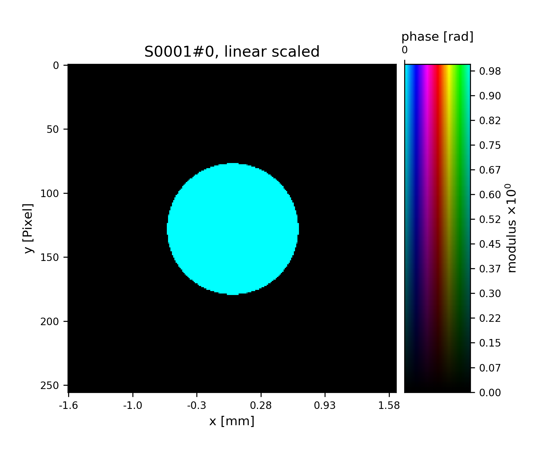
Fig. 6 Round test illumination (not necessarily smoothly varying).

or the coordinate grids from the Storage itself.

>>> pr3 = P.probe.new_storage(shape=pr_shape, psize=G.resolution)
>>> y, x = pr3.grids()
>>> apert = u.smooth_step(fsize[0]/5-np.abs(x), 3e-5)*u.smooth_step(fsize[1]/5-np.abs(y), 3e-5)
>>> pr3.fill(apert)
>>> fig = u.plot_storage(pr3, 2)

See Fig. 7 for the plotted image.

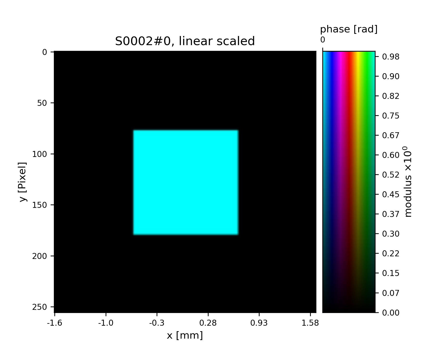
Fig. 7 Square test illumination.

In order to put some physics in the illumination we set the number of photons to 1 billion

>>> for pp in [pr, pr2, pr3]:
>>>     pp.data *= np.sqrt(1e9/np.sum(pp.data*pp.data.conj()))

>>> print(u.norm2(pr.data))
1000000000.0000001

and we quickly check if the propagation works.

>>> ill = pr.data[0]
>>> propagated_ill = G.propagator.fw(ill)
>>> fig = plt.figure(3)
>>> ax = fig.add_subplot(111)
>>> im = ax.imshow(np.log10(np.abs(propagated_ill)+1))
>>> plt.colorbar(im)

See Fig. 8 for the plotted image.

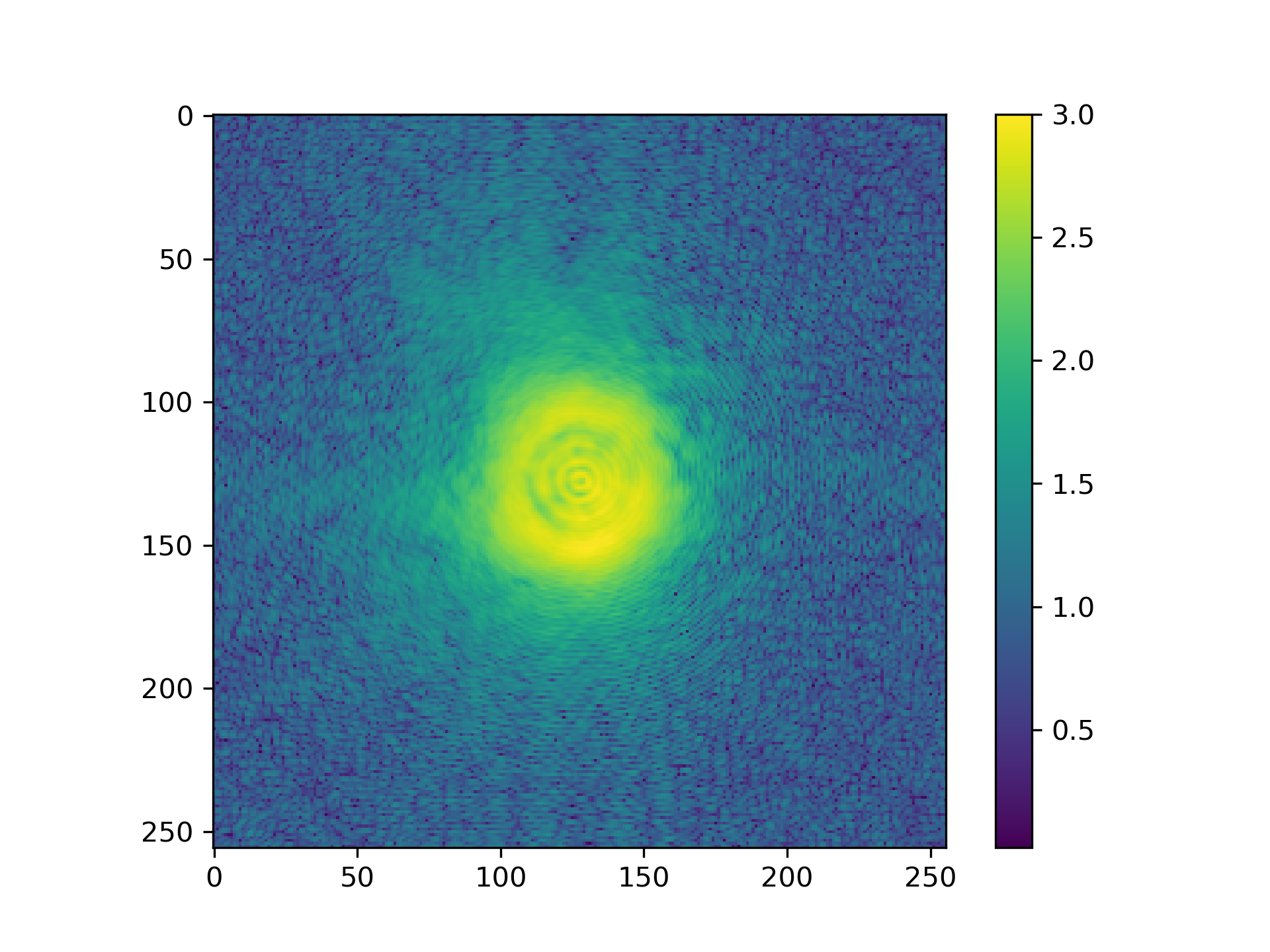
Fig. 8 Logarithmic intensity of propagated illumination.

Create scan pattern and object

We use the ptypy.core.xy module to create a scan pattern.

>>> pos = u.Param()
>>> pos.model = "round"
>>> pos.spacing = fsize[0]/8
>>> pos.steps = None
>>> pos.extent = fsize*1.5
>>> from ptypy.core import xy
>>> positions = xy.from_pars(pos)
>>> fig = plt.figure(4)
>>> ax = fig.add_subplot(111)
>>> ax.plot(positions[:, 1], positions[:, 0], 'o-')

See Fig. 9 for the plotted image.

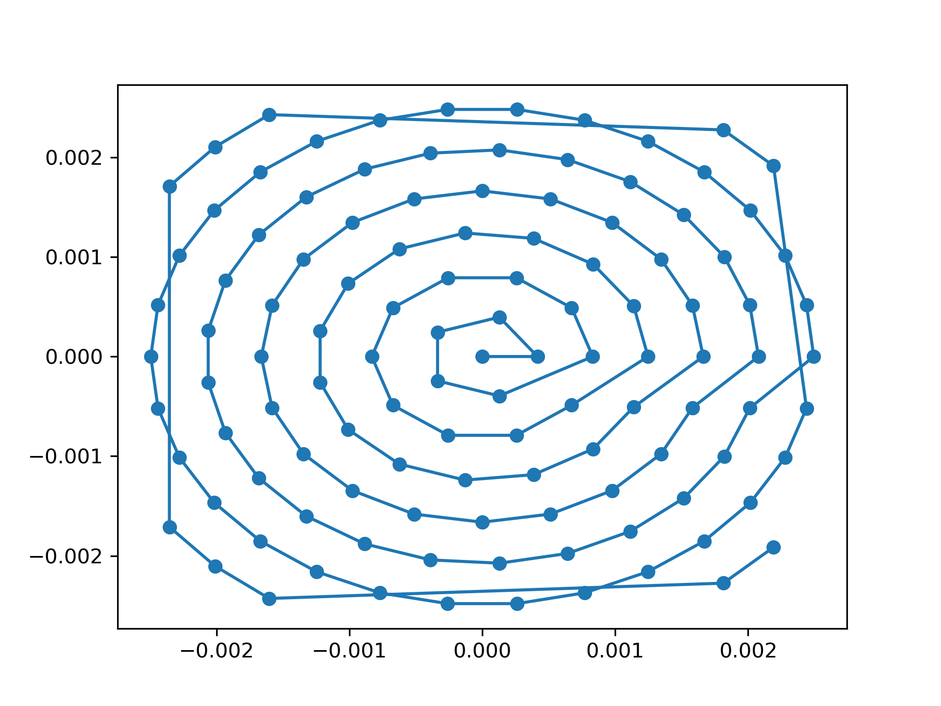
Fig. 9 Created scan pattern.

Next, we need to model a sample through an object transmisson function. We start of with a suited container which we call obj.

>>> P.obj = Container(P, 'Cobj', data_type='complex')

As we have learned from the previous Tutorial: Data access - Storage, View, Container, we can use View‘s to create a Storage data buffer of the right size.

>>> oar = View.DEFAULT_ACCESSRULE.copy()
>>> oar.storageID = 'S00'
>>> oar.psize = G.resolution
>>> oar.layer = 0
>>> oar.shape = G.shape
>>> oar.active = True

>>> for pos in positions:
>>>     # the rule
>>>     r = oar.copy()
>>>     r.coord = pos
>>>     V = View(P.obj, None, r)
>>>

We let the Storages in P.obj reformat in order to include all Views. Conveniently, this can be initiated from the top with Container.reformat()

>>> P.obj.reformat()
>>> print(P.obj.formatted_report())
(C)ontnr : Memory : Shape            : Pixel size      : Dimensions      : Views
(S)torgs : (MB)   : (Pixel)          : (meters)        : (meters)        : act.
--------------------------------------------------------------------------------
Cobj     :    6.5 : complex128
S00      :    6.5 :    1 * 638 * 640 :      1.3*1.3e-5 :      8.3*8.3e-3 :   116

At last we fill the object Storage S00 with a complex transmission. Again there is a convenience transmission function in the resources

>>> from ptypy.resources import flower_obj
>>> storage = P.obj.storages['S00']
>>> storage.fill(flower_obj(storage.shape[-2:]))
>>> fig = u.plot_storage(storage, 5)

See Fig. 10 for the plotted image.

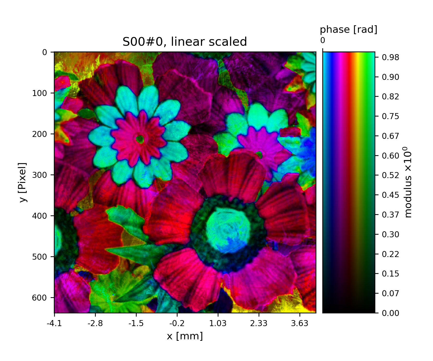
Fig. 10 Complex transmission function of the object.

Creating additional Views and the PODs

A single coherent propagation in PtyPy is represented by an instance of the POD class.

>>> print(POD.__doc__)

    POD : Ptychographic Object Descriptor

    A POD brings together probe view, object view and diff view. It also
    gives access to "exit", a (coherent) exit wave, and to propagation
    objects to go from exit to diff space.


>>> print(POD.__init__.__doc__)

        Parameters
        ----------
        ptycho : Ptycho
            The instance of Ptycho associated with this pod.

        model : ~ptypy.core.manager.ScanModel
            The instance of ScanModel (or it subclasses) which describes
            this pod.

        ID : str or int
            The pod ID, If None it is managed by the ptycho.

        views : dict or Param
            The views. See :py:attr:`DEFAULT_VIEWS`.

        geometry : Geo
            Geometry class instance and attached propagator

For creating a single POD we need a View to probe, object, exit wave and diffraction containers as well as the Geo class instance which represents the experimental setup.

First we create the missing Container’s.

>>> P.exit = Container(P, 'Cexit', data_type='complex')
>>> P.diff = Container(P, 'Cdiff', data_type='real')
>>> P.mask = Container(P, 'Cmask', data_type='real')

We start with one POD and its views.

>>> objviews = list(P.obj.views.values())
>>> obview = objviews[0]

We construct the probe View.

>>> probe_ar = View.DEFAULT_ACCESSRULE.copy()
>>> probe_ar.psize = G.resolution
>>> probe_ar.shape = G.shape
>>> probe_ar.active = True
>>> probe_ar.storageID = pr.ID
>>> prview = View(P.probe, None, probe_ar)

We construct the exit wave View. This construction is shorter as we only change a few bits in the access rule.

>>> exit_ar = probe_ar.copy()
>>> exit_ar.layer = 0
>>> exit_ar.active = True
>>> exview = View(P.exit, None, exit_ar)

We construct diffraction and mask Views. Even shorter is the construction of the mask View as, for the mask, we are essentially using the same access as for the diffraction data.

>>> diff_ar = probe_ar.copy()
>>> diff_ar.layer = 0
>>> diff_ar.active = True
>>> diff_ar.psize = G.psize
>>> mask_ar = diff_ar.copy()
>>> maview = View(P.mask, None, mask_ar)
>>> diview = View(P.diff, None, diff_ar)

Now we can create the POD.

>>> pods = []
>>> views = {'probe': prview, 'obj': obview, 'exit': exview, 'diff': diview, 'mask': maview}
>>> pod = POD(P, ID=None, views=views, geometry=G)
>>> pods.append(pod)

The POD is the most important class in PtyPy. Its instances are used to write the reconstruction algorithms using its attributes as local references. For example we can create and store an exit wave in the following convenient fashion:

>>> pod.exit = pod.probe * pod.object

The result of the calculation above is stored in the appropriate storage of P.exit. Therefore we can use this command to plot the result.

>>> exit_storage = list(P.exit.storages.values())[0]
>>> fig = u.plot_storage(exit_storage, 6)

See Fig. 11 for the plotted image.

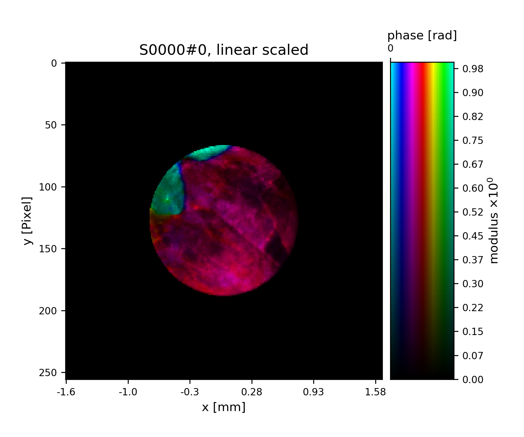
Fig. 11 Simulated exit wave using a pod.

The diffraction plane is also conveniently accessible with

>>> pod.diff = np.abs(pod.fw(pod.exit))**2

The result is stored in the diffraction container.

>>> diff_storage = list(P.diff.storages.values())[0]
>>> fig = u.plot_storage(diff_storage, 7, modulus='log')

See Fig. 12 for the plotted image.

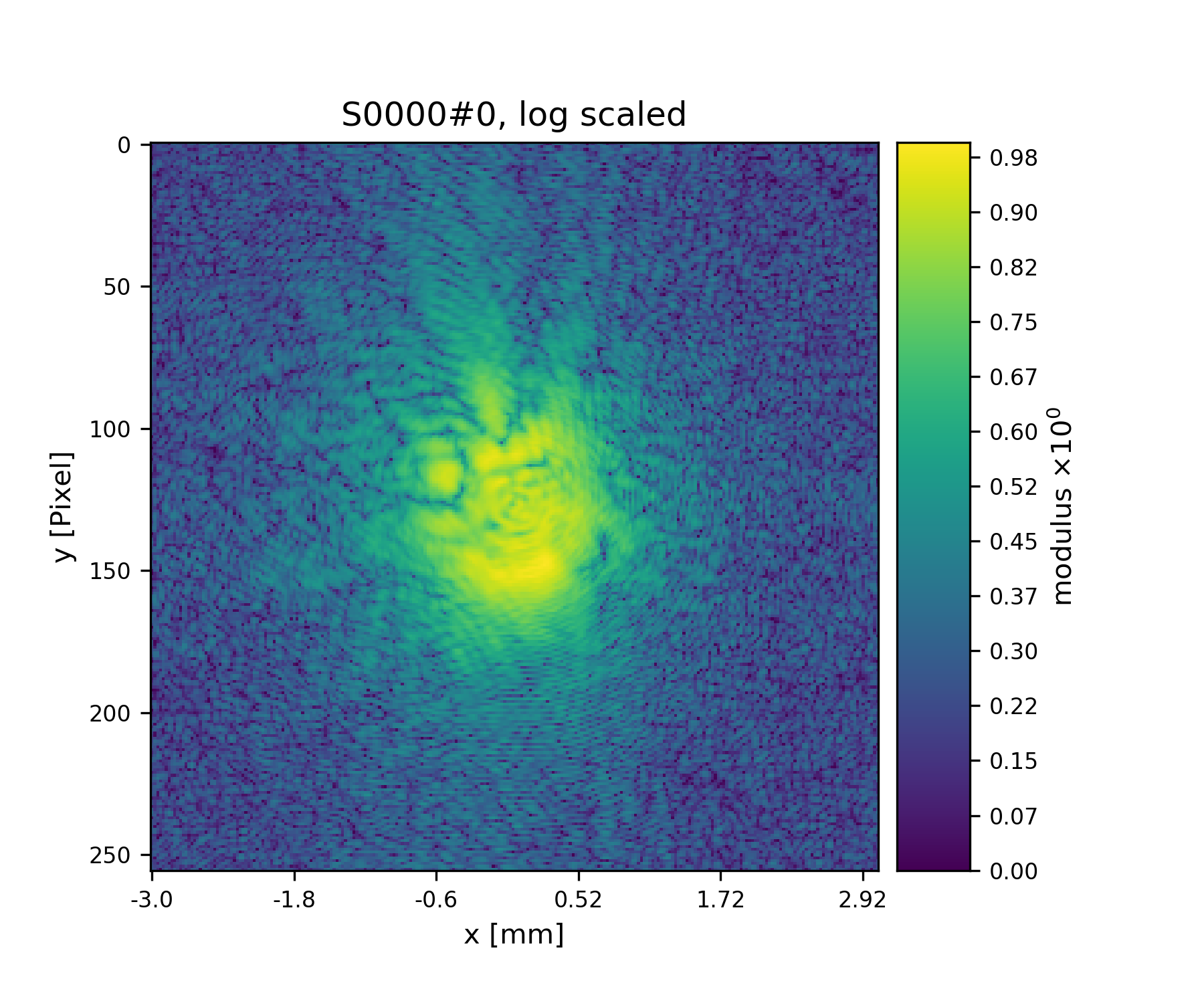
Fig. 12 First simulated diffraction image (without noise)

Creating the rest of the pods is now straight-forward since the data accesses are similar.

>>> for obview in objviews[1:]:
>>>     # we keep the same probe access
>>>     prview = View(P.probe, None, probe_ar)
>>>     # For diffraction and exit wave we need to increase the
>>>     # layer index as there is a new exit wave and diffraction pattern for each
>>>     # scan position
>>>     exit_ar.layer += 1
>>>     diff_ar.layer += 1
>>>     exview = View(P.exit, None, exit_ar)
>>>     maview = View(P.mask, None, mask_ar)
>>>     diview = View(P.diff, None, diff_ar)
>>>     views = {'probe': prview, 'obj': obview, 'exit': exview, 'diff': diview, 'mask': maview}
>>>     pod = POD(P, ID=None, views=views, geometry=G)
>>>     pods.append(pod)
>>>

We let the storage arrays adapt to the new Views.

>>> for C in [P.mask, P.exit, P.diff, P.probe]:
>>>     C.reformat()
>>>

And the rest of the simulation fits in three lines of code!

>>> for pod in pods:
>>>     pod.exit = pod.probe * pod.object
>>>     # we use Poisson statistics for a tiny bit of realism in the
>>>     # diffraction images
>>>     pod.diff = np.random.poisson(np.abs(pod.fw(pod.exit))**2)
>>>     pod.mask = np.ones_like(pod.diff)
>>>
>>>

We make a quick check on the diffraction patterns

>>> fig = u.plot_storage(diff_storage, 8, slices=':2,:,:', modulus='log')

See Fig. 13 for the plotted image.

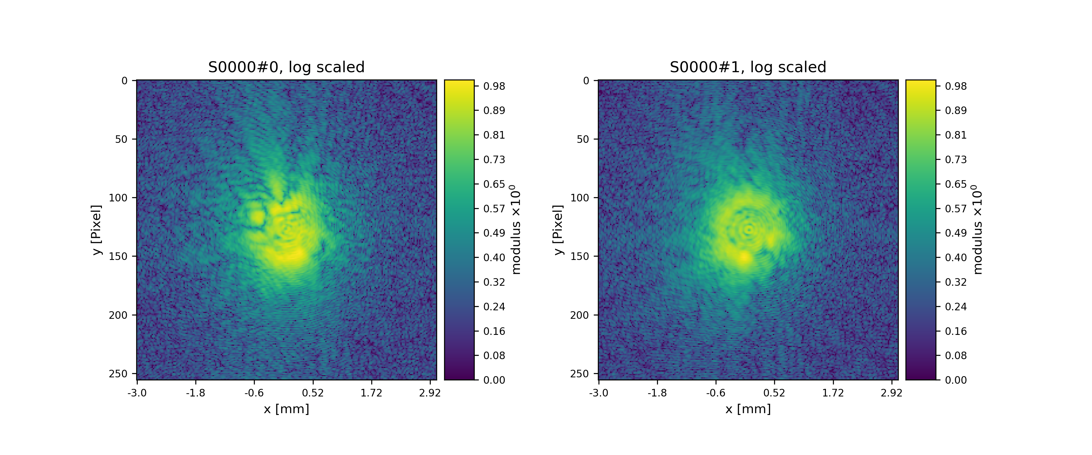
Fig. 13 Diffraction patterns with poisson statistics.

Well done! We can move forward to create and run a reconstruction engine as in section A basic Difference-Map implementation in Tutorial: A reconstruction engine from scratch or store the generated diffraction patterns as in the next section.

Storing the simulation

On unix system we choose the /tmp folder

>>> save_path = '/tmp/ptypy/sim/'
>>> import os

>>> if not os.path.exists(save_path):
>>>     os.makedirs(save_path)
>>>

First, we save the geometric info in a text file.

>>> with open(save_path+'geometry.txt', 'w') as f:
>>>     f.write('distance %.4e\n' % G.p.distance)
>>>     f.write('energy %.4e\n' % G.energy)
>>>     f.write('psize %.4e\n' % G.psize[0])
>>>     f.write('shape %d\n' % G.shape[0])
>>>     f.close()
>>>

Next, we save positions and the diffraction images. We don’t burden ourselves for now with converting to an image file format such as .tiff or a data format like .hdf5 but instead we use numpy’s binary storage format.

>>> with open(save_path+'positions.txt', 'w') as f:
>>>     if not os.path.exists(save_path+'ccd/'):
>>>         os.mkdir(save_path+'ccd/')
>>>     for pod in pods:
>>>         diff_frame = 'ccd/diffraction_%04d.npy' % pod.di_view.layer
>>>         f.write(diff_frame+' %.4e %.4e\n' % tuple(pod.ob_view.coord))
>>>         frame = pod.diff.astype(np.int32)
>>>         np.save(save_path+diff_frame, frame)
>>>

If you want to learn how to convert this “experiment” into ptypy data file (.ptyd), see to Tutorial : Subclassing PtyScan

Tutorial: A reconstruction engine from scratch

Note

This tutorial was generated from the python source [ptypy_root]/tutorial/ownengine.py using ptypy/doc/script2rst.py. You are encouraged to modify the parameters and rerun the tutorial with:

$ python [ptypy_root]/tutorial/ownengine.py

In this tutorial, we want to provide the information needed to create an engine compatible with the state mixture expansion of ptychogrpahy as described in Thibault et. al 2013 1 .

First we import ptypy and the utility module

>>> import ptypy
>>> from ptypy import utils as u
>>> import numpy as np

Preparing a managing Ptycho instance

We need to prepare a managing Ptycho instance. It requires a parameter tree, as specified in Parameter tree structure

First, we create a most basic input paramater tree. There are many default values, but we specify manually only a more verbose output and single precision for the data type.

>>> p = u.Param()
>>> p.verbose_level = 3
>>> p.data_type = "single"

Now, we need to create a set of scans that we wish to reconstruct in the reconstruction run. We will use a single scan that we call ‘MF’ and mark the data source as ‘test’ to use the PtyPy internal MoonFlowerScan

>>> p.scans = u.Param()
>>> p.scans.MF = u.Param()
>>> p.scans.MF.name = 'Full'
>>> p.scans.MF.data = u.Param()
>>> p.scans.MF.data.name = 'MoonFlowerScan'
>>> p.scans.MF.data.shape = 128
>>> p.scans.MF.data.num_frames = 400

This bare parameter tree will be the input for the Ptycho class which is constructed at level=2. It means that it creates all necessary basic Container instances like probe, object diff , etc. It also loads the first chunk of data and creates all View and POD instances, as the verbose output will tell.

>>> P = ptypy.core.Ptycho(p, level=2)

A quick look at the diffraction data

>>> diff_storage = list(P.diff.storages.values())[0]
>>> fig = u.plot_storage(diff_storage, 0, slices=(slice(2), slice(None), slice(None)), modulus='log')

See Fig. 14 for the plotted image.

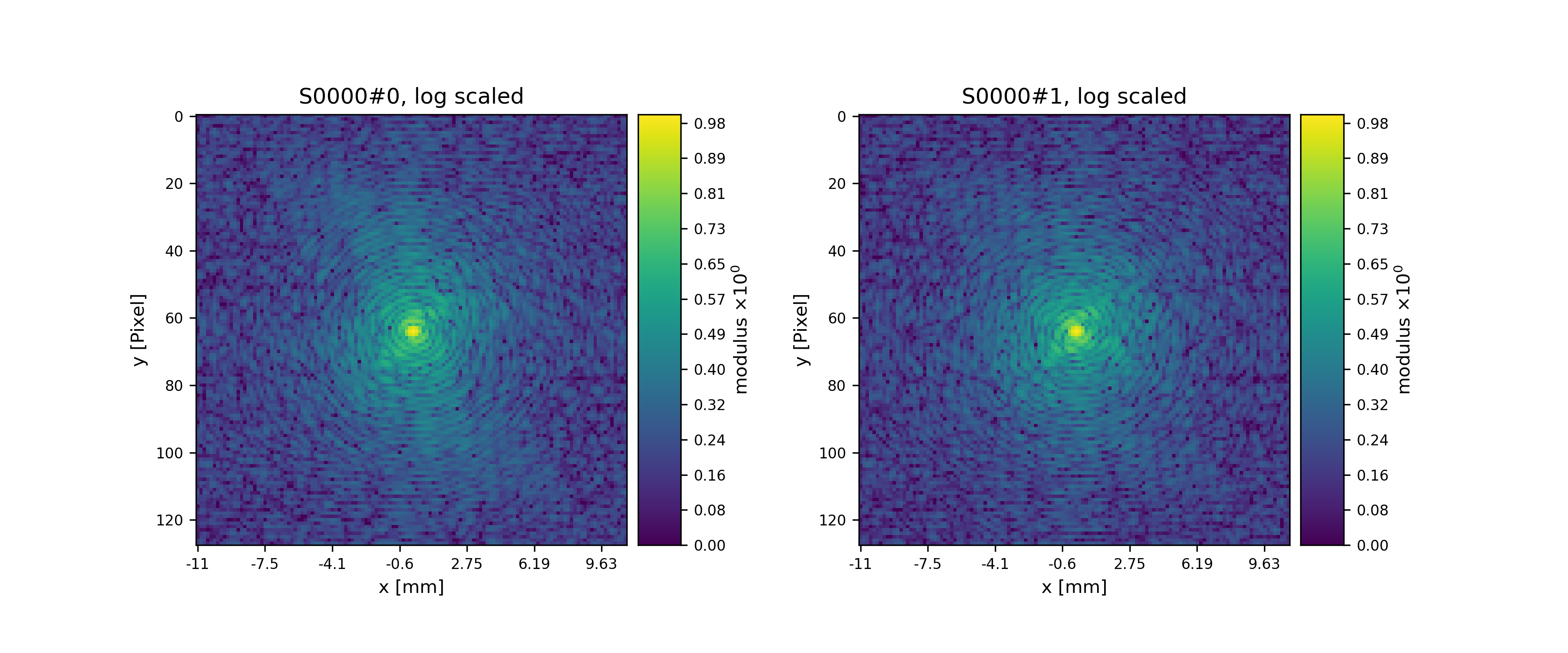
Fig. 14 Plot of simulated diffraction data for the first two positions.

We don’t need to use PtyPy’s Ptycho class to arrive at this point. The structure P that we arrive with at the end of Tutorial: Modeling the experiment - Pod, Geometry suffices completely.

Probe and object are not so exciting to look at for now. As default, probes are initialized with an aperture like support.

>>> probe_storage = list(P.probe.storages.values())[0]
>>> fig = u.plot_storage(list(P.probe.S.values())[0], 1)

See Fig. 15 for the plotted image.

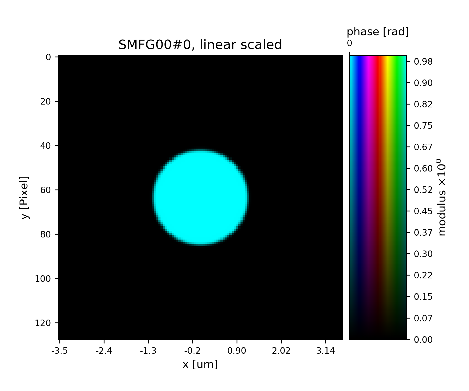
Fig. 15 Plot of the starting guess for the probe.

A basic Difference-Map implementation

Now we can start implementing a simple DM algorithm. We need three basic functions, one is the fourier_update that implements the Fourier modulus constraint.

\[\psi_{d,\lambda,k} = \mathcal{D}_{\lambda,z}^{-1}\left\{\sqrt{I_{d}}\frac{\mathcal{D}_{\lambda,z} \{\psi_{d,\lambda,k}\}}{\sum_{\lambda,k} |\mathcal{D}_{\lambda,z} \{\psi_{d,\lambda,k}\} |^2}\right\}\]

>>> def fourier_update(pods):
>>>     import numpy as np
>>>     pod = list(pods.values())[0]
>>>     # Get Magnitude and Mask
>>>     mask = pod.mask
>>>     modulus = np.sqrt(np.abs(pod.diff))
>>>     # Create temporary buffers
>>>     Imodel = np.zeros_like(pod.diff)
>>>     err = 0.
>>>     Dphi = {}
>>>     # Propagate the exit waves
>>>     for gamma, pod in pods.items():
>>>         Dphi[gamma] = pod.fw(2*pod.probe*pod.object - pod.exit)
>>>         Imodel += np.abs(Dphi[gamma] * Dphi[gamma].conj())
>>>     # Calculate common correction factor
>>>     factor = (1-mask) + mask * modulus / (np.sqrt(Imodel) + 1e-10)
>>>     # Apply correction and propagate back
>>>     for gamma, pod in pods.items():
>>>         df = pod.bw(factor*Dphi[gamma]) - pod.probe*pod.object
>>>         pod.exit += df
>>>         err += np.mean(np.abs(df*df.conj()))
>>>     # Return difference map error on exit waves
>>>     return err
>>>

>>> def probe_update(probe, norm, pods, fill=0.):
>>>     """
>>>     Updates `probe`. A portion `fill` of the probe is kept from
>>>     iteration to iteration. Requires `norm` buffer and pod dictionary
>>>     """
>>>     probe *= fill
>>>     norm << fill + 1e-10
>>>     for name, pod in pods.items():
>>>         if not pod.active: continue
>>>         probe[pod.pr_view] += pod.object.conj() * pod.exit
>>>         norm[pod.pr_view] += pod.object * pod.object.conj()
>>>     # For parallel usage (MPI) we have to communicate the buffer arrays
>>>     probe.allreduce()
>>>     norm.allreduce()
>>>     probe /= norm
>>>

>>> def object_update(obj, norm, pods, fill=0.):
>>>     """
>>>     Updates `object`. A portion `fill` of the object is kept from
>>>     iteration to iteration. Requires `norm` buffer and pod dictionary
>>>     """
>>>     obj *= fill
>>>     norm << fill + 1e-10
>>>     for pod in pods.values():
>>>         if not pod.active: continue
>>>         pod.object += pod.probe.conj() * pod.exit
>>>         norm[pod.ob_view] += pod.probe * pod.probe.conj()
>>>     obj.allreduce()
>>>     norm.allreduce()
>>>     obj /= norm
>>>

>>> def iterate(Ptycho, num):
>>>     # generate container copies
>>>     obj_norm = P.obj.copy(fill=0.)
>>>     probe_norm = P.probe.copy(fill=0.)
>>>     errors = []
>>>     for i in range(num):
>>>         err = 0
>>>         # fourier update
>>>         for di_view in Ptycho.diff.V.values():
>>>             if not di_view.active: continue
>>>             err += fourier_update(di_view.pods)
>>>         # probe update
>>>         probe_update(Ptycho.probe, probe_norm, Ptycho.pods)
>>>         # object update
>>>         object_update(Ptycho.obj, obj_norm, Ptycho.pods)
>>>         # print error
>>>         errors.append(err)
>>>         if i % 3==0: print(err)
>>>     # cleanup
>>>     P.obj.delete_copy()
>>>     P.probe.delete_copy()
>>>     #return error
>>>     return errors
>>>

We start off with a small number of iterations.

>>> iterate(P, 9)
438026.50735607144
315508.66172933887
237978.26703255248

We note that the error (here only displayed for 3 iterations) is already declining. That is a good sign. Let us have a look how the probe has developed.

>>> fig = u.plot_storage(list(P.probe.S.values())[0], 2)

See Fig. 16 for the plotted image.

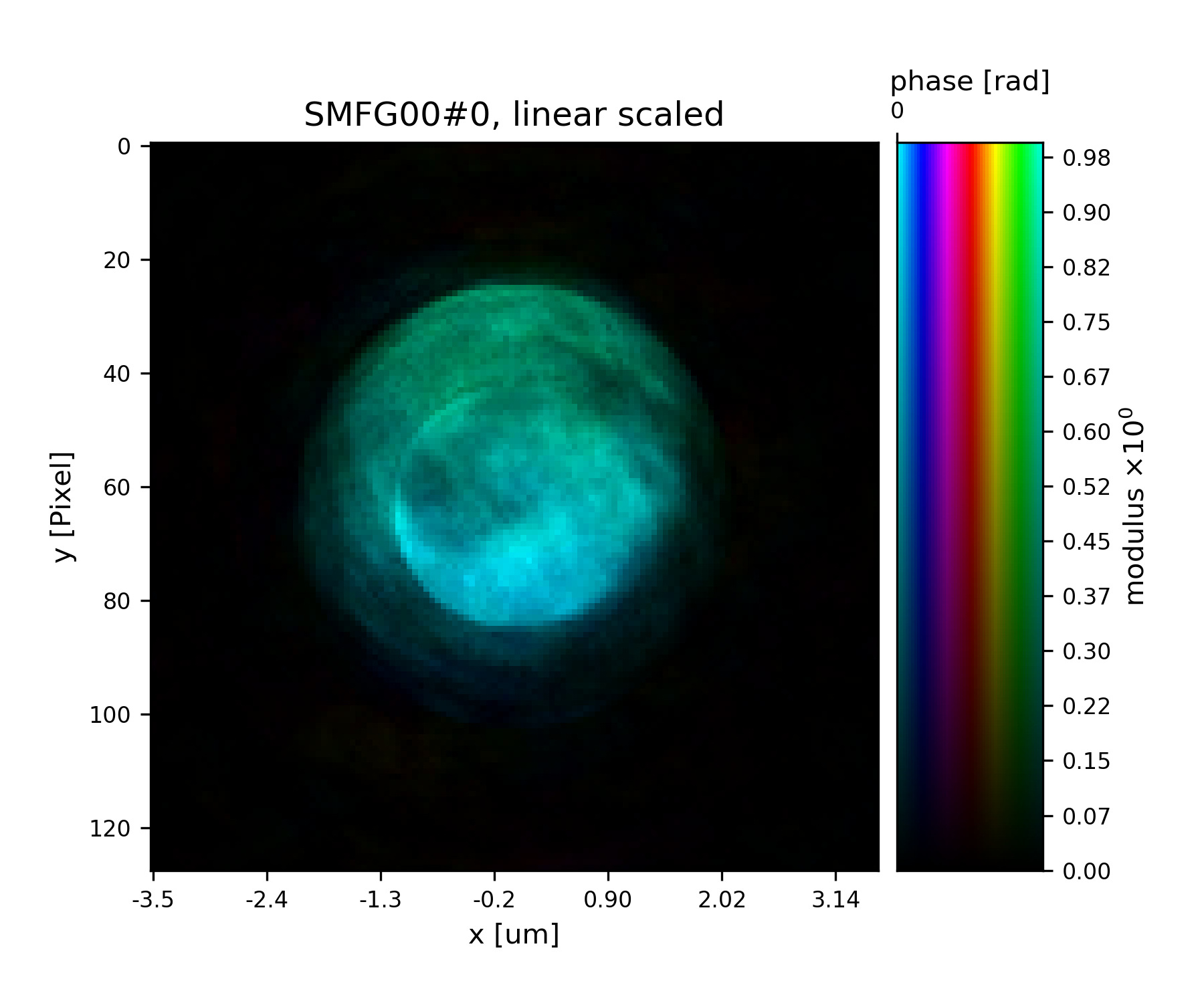
Fig. 16 Plot of the reconstructed probe after 9 iterations. We observe that the actaul illumination of the sample must be larger than the initial guess.

Looks like the probe is on a good way. How about the object?

>>> fig = u.plot_storage(list(P.obj.S.values())[0], 3, slices='0,120:-120,120:-120')

See Fig. 17 for the plotted image.

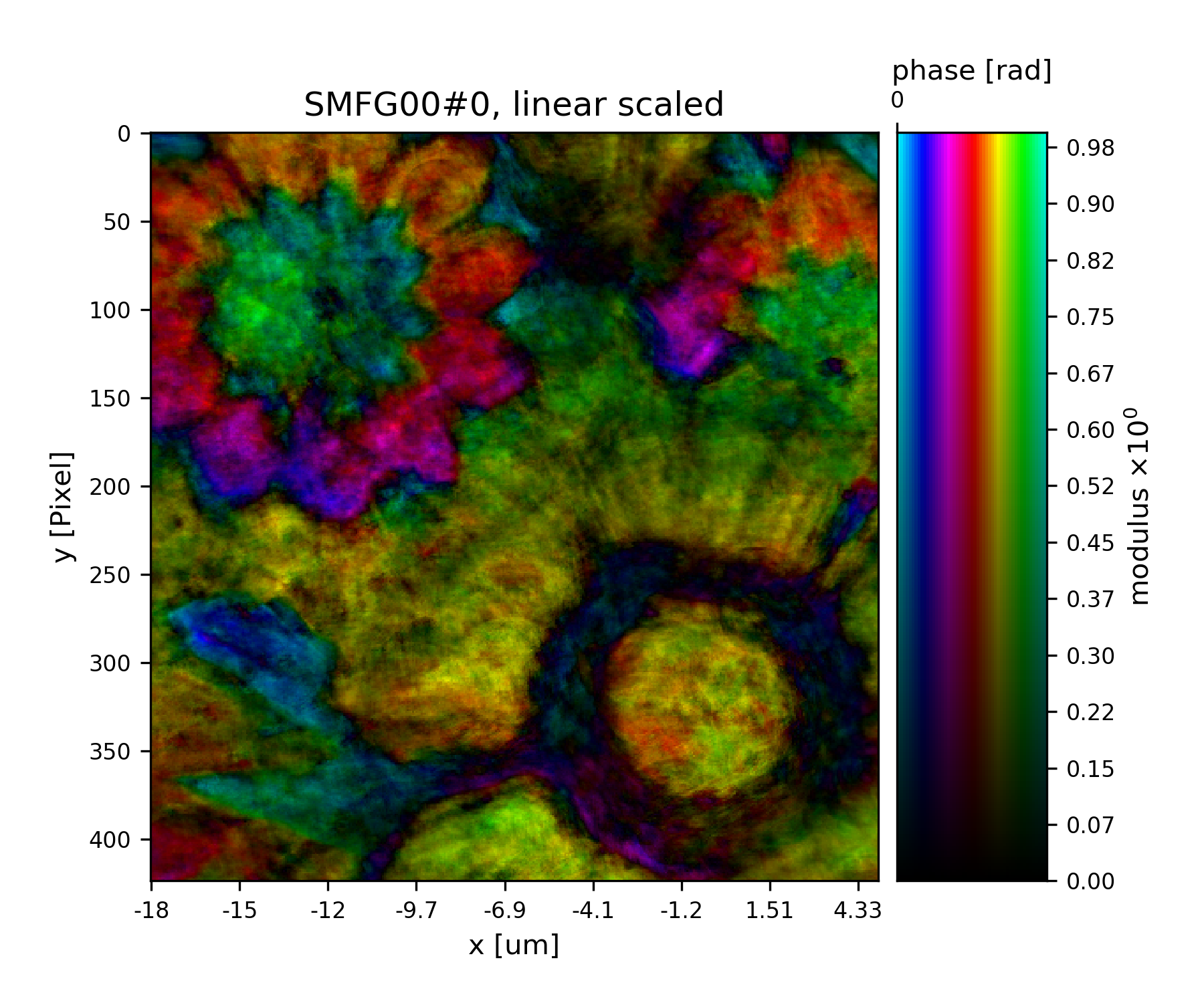
Fig. 17 Plot of the reconstructed object after 9 iterations. It is not quite clear what object is reconstructed

Ok, let us do some more iterations. 36 will do.

>>> iterate(P, 36)
158603.9740395377
91072.73033678501
61211.753241738574
46684.904276998306
37483.80987198136
28430.613557863566
22350.477334251234
19980.413638760696
18558.9012019789
17776.334601063198
17781.86195633913
17806.30507956264

Error is still on a steady descent. Let us look at the final reconstructed probe and object.

>>> fig = u.plot_storage(list(P.probe.S.values())[0], 4)

See Fig. 18 for the plotted image.

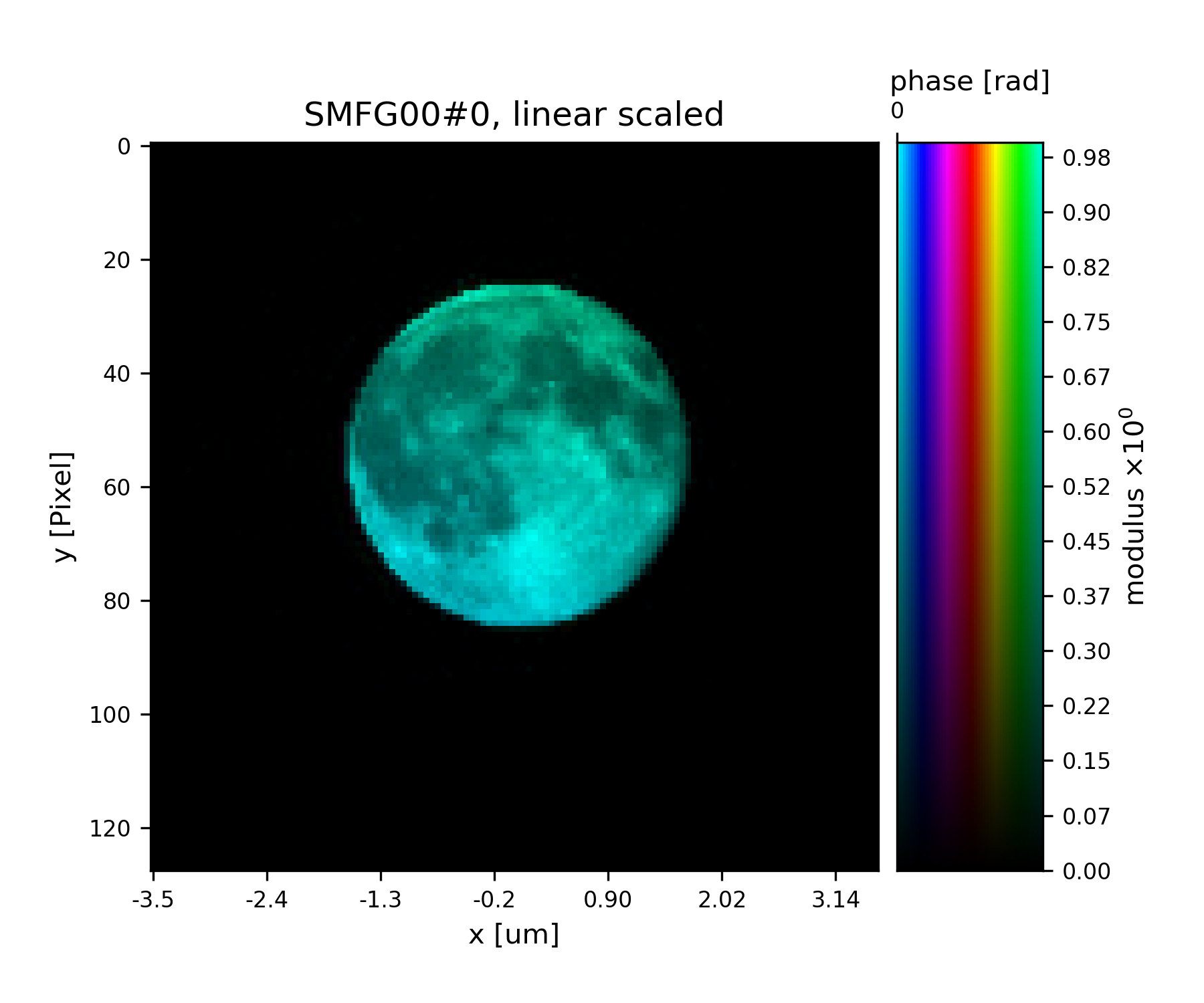
Fig. 18 Plot of the reconstructed probe after a total of 45 iterations. It’s a moon !

>>> fig = u.plot_storage(list(P.obj.S.values())[0], 5, slices='0,120:-120,120:-120')

See Fig. 19 for the plotted image.

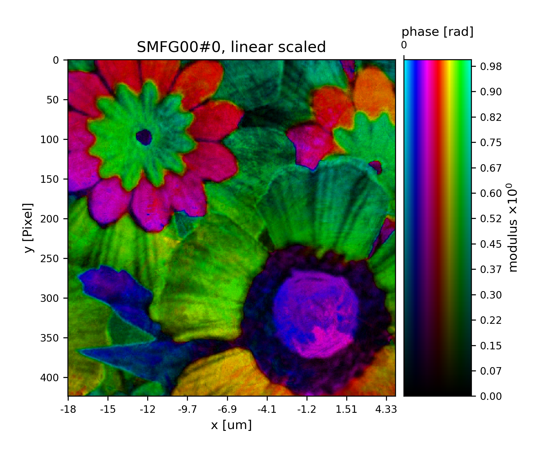
Fig. 19 Plot of the reconstructed object after a total of 45 iterations. It’s a bunch of flowers !

1

16. Thibault and A. Menzel, Nature 494, 68 (2013)