Working With Large Data#
Learning how to work with large experimental datasets using a block scan model and GPU acceleration.
All tutorials so far have been using either simulated data (MoonFlower) or experimental data specifically prepared and reduced in memory for the purpose of those tutorials. From now, we are going to look at full-sized data in exactly the format that it has been collected at the various instruments and microscopes. This means we should certainly use GPU-accelerated reconstruction engines and also adopt using the block scan models which are more efficient in dealing with large data.
The data#
Data file |
Type |
Download |
Courtesy of |
Reference |
|---|---|---|---|---|
i08-1-5776_cropped.h5 |
Raw |
Majid Kazemian |
At the I08-1 instrument at the Diamond Light Source, raw data is written into HDF5/Nexus files. As an example, we can look at the original raw data from the nanogold test sample which is stored in "dls_i08_nanogold_spiral/i08-1-5776_cropped.h5" and inspect the relevant entries
import h5py, os
tutorial_data_home = "../../data/"
dataset = "dls_i08_nanogold_spiral/i08-1-5776_cropped.h5"
path_to_data = os.path.join(tutorial_data_home, dataset)
with h5py.File(path_to_data) as f:
    keys = ["data", "posx", "posy"]
    print("The file {} has the following relevant entries: \n".format(path_to_data))
    print('\n'.join('\t* {0:<30} shape = {1:}'.format(k,f[k].shape) for k in keys))
for the diffraction intensities and the scan positions
The file ../../data/dls_i08_nanogold_spiral/i08-1-5776_cropped.h5 has the following relevant entries:

	* data                           shape = (1000, 1024, 1024)
	* posx                           shape = (1000,)
	* posy                           shape = (1000,)
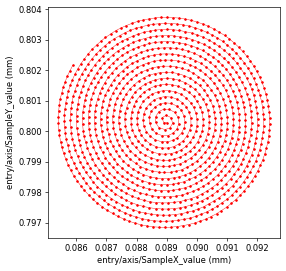
which follow a “spiral” trajectory where for each point along the spiral, the X and Y coordinate is saved in posx and posy, respectively

import h5py, os
tutorial_data_home = "../../data/"
dataset = "dls_i08_nanogold_spiral/i08-1-5776_cropped.h5"
path_to_data = os.path.join(tutorial_data_home, dataset)
with h5py.File(path_to_data) as f:
    keys = ["data", "posx", "posy"]
    print("The file {} has the following relevant entries: \n".format(path_to_data))
    print('\n'.join('\t* {0:<30} shape = {1:}'.format(k,f[k].shape) for k in keys))
Loading the data#
We use the Hdf5Loader for reading the data into PtyPy with orientation=2
p.scans.scan_00.data = u.Param()
p.scans.scan_00.data.name = 'Hdf5Loader'
p.scans.scan_00.data.orientation = 2
providing the path and key for the diffraction intensities
p.scans.scan_00.data.intensities = u.Param()
p.scans.scan_00.data.intensities.file = path_to_data
p.scans.scan_00.data.intensities.key = "data"
and the slow/fast axis of the scan positions:
p.scans.scan_00.data.positions = u.Param()
p.scans.scan_00.data.positions.file = path_to_data
p.scans.scan_00.data.positions.slow_key = "posy"
p.scans.scan_00.data.positions.slow_multiplier = 1e-3
p.scans.scan_00.data.positions.fast_key = "posx"
p.scans.scan_00.data.positions.fast_multiplier = 1e-3
Instead of loading the entire scan which has \(1000\) scan points, we can limit ourselves to the first \(900\) positions using bounding_box.fast_axis_bounds:
p.scans.scan_00.data.positions.bounding_box = u.Param()
p.scans.scan_00.data.positions.bounding_box.fast_axis_bounds = [0,900]
The raw data collected at I08-1 also needs to be corrected for the dark current, which can be achieved by loading a darkfield image
p.scans.scan_00.data.darkfield = u.Param()
p.scans.scan_00.data.darkfield.file = path_to_data
p.scans.scan_00.data.darkfield.key = "dark"
that will be subtracted from each loaded diffraction pattern inside the Hdf5Loader class. Finally, we need to provide the correct meta information (energy, distance, pixel size)
p.scans.scan_00.data.energy = 0.710
p.scans.scan_00.data.distance = 0.072
p.scans.scan_00.data.psize = 11e-6
and we can specify a shape smaller or equal to the original shape of the data (1024x1024) as well as rebin=2
p.scans.scan_00.data.shape = (1024,1024)
p.scans.scan_00.data.rebin = 2
p.scans.scan_00.data.auto_center = True
which will load the data with a shape of (1024,1024) and bin the resulting frames into a final shape of (512,512). For this particular example, these operations are save to do without loosing any relevant information in the diffraction data.
The scan model#
For this example, it is best to use the "BlockFull" scan model
p.scans = u.Param()
p.scans.scan_00 = u.Param()
p.scans.scan_00.name = 'BlockFull'
with a block size defined by frames_per_block of \(100\)
p.frames_per_block = 100
which will load in the data frames in chunks of \(100\) and then does all the processing on the GPU over the entire block which provides a boost in performance since compuations within each block can be distributed over many GPU threads.
Reconstruction engine#
For the reconstruction we use the difference map (DM) engine the set of paramters most commonly used for the I08-1 instrument
p.engines = u.Param()
p.engines.engine = u.Param()
p.engines.engine.name = "DM_cupy"
p.engines.engine.numiter = 200
p.engines.engine.numiter_contiguous = 10
p.engines.engine.probe_support = None
p.engines.engine.probe_update_start = 0
p.engines.engine.probe_fourier_support = None
p.engines.engine.record_local_error = False
p.engines.engine.alpha = 0.95
p.engines.engine.fourier_power_bound = 0.25
p.engines.engine.overlap_converge_factor = 0.001
p.engines.engine.overlap_max_iterations = 20
p.engines.engine.update_object_first = False
p.engines.engine.obj_smooth_std = 20
p.engines.engine.object_inertia = 0.001
p.engines.engine.probe_inertia = 0.001
p.engines.engine.clip_object = [0,1]
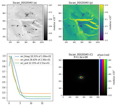
resulting in a reconstruction of the nanogold sample after \(200\) iterations

Challenge
Modify data loading (e.g. rebin or shape) parameters and engine parameters (e.g. fourier_power_bound or overlap_converge_factor) and observe if/how it improves the quality, convergence or speed of the reconstruction.
import ptypy, os
import ptypy.utils as u

# This will import the HDF5Loader class
ptypy.load_ptyscan_module("hdf5_loader")

# This will import the GPU engines
ptypy.load_gpu_engines("cupy")

# Root directory of tutorial data
tutorial_data_home = "../../data/"

# Dataset for this tutorial
dataset = "dls_i08_nanogold_spiral/i08-1-5776_cropped.h5"

# Absolute path to HDF5 file with raw data
path_to_data = os.path.join(tutorial_data_home, dataset)

# Create parameter tree
p = u.Param()

# Set verbose level to info
p.verbose_level = "interactive"

# Scan label
p.run = "dls_i08_nanogold"

# Data loading and processing should
# happen in chunks of this size
p.frames_per_block = 100

# Set io settings (no files saved)
p.io = u.Param()
p.io.rfile = None
p.io.autosave = u.Param(active=False)
p.io.interaction = u.Param(active=False)

# Live-plotting during the reconstruction
p.io.autoplot = u.Param()
p.io.autoplot.active=True
p.io.autoplot.threaded = False
p.io.autoplot.layout = "jupyter"
p.io.autoplot.interval = 10

# Define the scan model
p.scans = u.Param()
p.scans.scan_00 = u.Param()
p.scans.scan_00.name = 'BlockFull'

# Initial illumination (based on simulated optics)
p.scans.scan_00.illumination = u.Param()
p.scans.scan_00.illumination.model = None
p.scans.scan_00.illumination.photons = None
p.scans.scan_00.illumination.aperture = u.Param()
p.scans.scan_00.illumination.aperture.form = "circ"
p.scans.scan_00.illumination.aperture.size = 333e-6
p.scans.scan_00.illumination.propagation = u.Param()
p.scans.scan_00.illumination.propagation.focussed = 13.725e-3
p.scans.scan_00.illumination.propagation.parallel = 45e-6
p.scans.scan_00.illumination.propagation.antialiasing = 1
p.scans.scan_00.illumination.diversity = u.Param()
p.scans.scan_00.illumination.diversity.power = 0.1
p.scans.scan_00.illumination.diversity.noise = [0.5,1.0]

# Initial object
p.scans.scan_00.sample = u.Param()
p.scans.scan_00.sample.model = None
p.scans.scan_00.sample.diversity = None
p.scans.scan_00.sample.process = None

# Coherence parameters (modes)
p.scans.scan_00.coherence = u.Param()
p.scans.scan_00.coherence.num_probe_modes = 1
p.scans.scan_00.coherence.num_object_modes = 1

# Data loader
p.scans.scan_00.data = u.Param()
p.scans.scan_00.data.name = 'Hdf5Loader'
p.scans.scan_00.data.orientation = 2

p.scans.scan_00.data.intensities = u.Param()
p.scans.scan_00.data.intensities.file = path_to_data
p.scans.scan_00.data.intensities.key = "data"

p.scans.scan_00.data.positions = u.Param()
p.scans.scan_00.data.positions.file = path_to_data
p.scans.scan_00.data.positions.slow_key = "posy"
p.scans.scan_00.data.positions.slow_multiplier = 1e-3
p.scans.scan_00.data.positions.fast_key = "posx"
p.scans.scan_00.data.positions.fast_multiplier = 1e-3
p.scans.scan_00.data.positions.bounding_box = u.Param()
p.scans.scan_00.data.positions.bounding_box.fast_axis_bounds = [0,900]

p.scans.scan_00.data.darkfield = u.Param()
p.scans.scan_00.data.darkfield.file = path_to_data
p.scans.scan_00.data.darkfield.key = "dark"

p.scans.scan_00.data.energy = 0.710
p.scans.scan_00.data.distance = 0.072
p.scans.scan_00.data.psize = 11e-6
p.scans.scan_00.data.shape = (1024,1024)
p.scans.scan_00.data.rebin = 2
p.scans.scan_00.data.auto_center = True

# Reconstruct using GPU-accelerated DM
p.engines = u.Param()
p.engines.engine = u.Param()
p.engines.engine.name = "DM_cupy"
p.engines.engine.numiter = 200
p.engines.engine.numiter_contiguous = 10
p.engines.engine.probe_support = None
p.engines.engine.probe_update_start = 0
p.engines.engine.probe_fourier_support = None
p.engines.engine.record_local_error = False
p.engines.engine.alpha = 0.95
p.engines.engine.fourier_power_bound = 0.25
p.engines.engine.overlap_converge_factor = 0.001
p.engines.engine.overlap_max_iterations = 20
p.engines.engine.update_object_first = False
p.engines.engine.obj_smooth_std = 20
p.engines.engine.object_inertia = 0.001
p.engines.engine.probe_inertia = 0.001
p.engines.engine.clip_object = [0,1]

# Run reconstruction
P = ptypy.core.Ptycho(p,level=5)


