Working with Data from SOLEIL - the SWING beamline#
Learning how to reconstruct from scratch with collected at SWING - courtesy of Javier Perez
Imagine the following scenario: You have been given a fresh ptychographic data set to reconstruct but you don’t have all the details about the instrument the data was collected at or the structure of the raw data file. This can often be the reality for users of ptychography at synchrotrons or anybody who is tasked with supporting the analysis of a ptychographic data set. This tutorial is aiming to provide a rough guide on how to approach such from scratch reconstruction based on a Siemens Star data set provide by Javier Perez from the SWING beamline at SOLEIL in preparation for the PtyPy 2025 workshop.
Data inspection via tree search#
Data file |
Type |
Download |
Courtesy of |
Reference |
|---|---|---|---|---|
nanoprobe3d_centrage_00031_2024-12-13_11-14-18.h5 |
Raw data |
Javier Perez |
||
nanoprobe3d_centrage_00032_2024-12-13_11-25-06.h5 |
Raw data |
Javier Perez |
There are two independent raw data files in HDF5 format which supposedly contain all the relevant information but the file structure is unknown. So first, we are trying to poke around a bit and inspect HDF5 files. The following snippet does a nested search and prints keys, shapes and types of datasets:
def tree_search(group):
    for k,v in group.items():
        print(f"group = {v.name}")
        if isinstance(v, h5py.Dataset):
            data = v[()]
            if isinstance(data, np.bytes_):
                print(f"\t{v.name} | data: {str(data)}")
            elif len(data) > 1:
                print(f"\t{v.name} | shape: {v.shape} | dtype: {v.dtype}")
            else:
                print(f"\t{v.name} | data: {data[0]}")
        elif isinstance(v, h5py.Group):
            tree_search(v)

with h5py.File(path_to_data, "r") as f:
    tree_search(f)
import h5py, os
import numpy as np

tutorial_data_home = "../../data/"
scan_nr = 32
#dataset = f"soleil_swing_siemens/nanoprobe3d_centrage_{scan_nr:05d}_2024-12-13_11-14-18.h5"
dataset = f"soleil_swing_siemens/nanoprobe3d_centrage_{scan_nr:05d}_2024-12-13_11-25-06.h5"
path_to_data = os.path.join(tutorial_data_home, dataset)

def tree_search(group):
    for k,v in group.items():
        #print(f"group = {v.name}")
        if isinstance(v, h5py.Dataset):
            data = v[()]
            if isinstance(data, np.bytes_):
                #print(f"\t{v.name} | data: {str(data)}")
                pass
            elif len(data) > 1:
                print(f"\t{v.name} | shape: {v.shape} | dtype: {v.dtype}")
                pass
            else:
                print(f"\t{v.name} | data: {data[0]}")
                pass
        elif isinstance(v, h5py.Group):
            tree_search(v)

with h5py.File(path_to_data, "r") as f:
    tree_search(f)
Finding the required bits of information#
In order to attempt a successful reconstruction, we need
an array/list of diffraction patterns
an array/list of scanning positions
experimental properties (sample-detector distance, detector pixelsize, photon energy)
By inspecting the HDF5 file, we can determine that the detector was an EIGER 4M with its pixel size and distance saved as /SiemensStar_00032/SWING/EIGER-4M/pixel_size_x and /SiemensStar_00032/SWING/EIGER-4M/distance respectively. The diffraction data seems to be located at /SiemensStar_00032/scan_data/eiger_image.
The scan_data section also seems to have a list of sample positions labelled /SiemensStar_00032//scan_data/calc_gated_sample_tx and /SiemensStar_00032//scan_data/calc_gated_sample_tx, and digging a bit further into the tree we can find /SiemensStar_00032//SWING/i11-c-c03__op__mono/energy which seems to provide us with the photon energy that is saved by the monochromator. In full we have identified the following entries in the HDF5 file:
# Keys to data and metadata
root_entry = f"/SiemensStar_{scan_nr:05d}"
data_key = f"/{root_entry}/scan_data/eiger_image"
det_pixsize_key = f"/{root_entry}/SWING/EIGER-4M/pixel_size_x"
det_distance_key = f"/{root_entry}/SWING/EIGER-4M/distance"
sample_posx_key = f"/{root_entry}/scan_data/calc_gated_sample_tx"
sample_posz_key = f"/{root_entry}/scan_data/calc_gated_sample_tz"
photon_energy_key = f"/{root_entry}/SWING/i11-c-c03__op__mono/energy"
Loading data into memory and inspecting metadata#
It is now time to look at the data a bit more closely. First, we load everything into memory and print out some overall information:
with h5py.File(path_to_data, "r") as f:
    data = f[data_key][:]
    posx = f[sample_posx_key][:]
    posz = f[sample_posz_key][:]
    photon_energy_kev = f[photon_energy_key][0]
    det_pixsize_um = f[det_pixsize_key][0]
    det_distance_mm = f[det_distance_key][0]
print(f"Nr. of points: {data.shape[0]}, \
        Detector shape: {data[0].shape}, \
        Energy: {photon_energy_kev:.1f} keV, \
        Detector distance: {det_distance_mm:.1f} mm, \
        Detector pixelsize: {det_pixsize_um} um")
This gives us the following output:
Nr. of points: 632, Detector shape: (1000, 1000), Energy: 8.0 keV, Detector distance: 6491.3 mm, Detector pixelsize: 75.0 um
and suggests that we have a scan with \(632\) points each with diffraction patterns of shape \(1000 x 1000\) pixels. The pixel size is \(75\), the detector distance \(6491.3\) and the photon energy \(8\). Knowing that SWING is a hard-xray beamline and looking at the technical facts provided on the beamline’s website we can safely assume that the pixel size is \(75\) microns, the distance is \(6491.3\) mm and the photon energy is \(8\) keV.
with h5py.File(path_to_data, "r") as f:
    data = f[data_key][:]
    posx = f[sample_posx_key][:]
    posz = f[sample_posz_key][:]
    photon_energy_kev = f[photon_energy_key][0]
    det_pixsize_um = f[det_pixsize_key][0]
    det_distance_mm = f[det_distance_key][0]
print(f"Nr. of points: {data.shape[0]}, \
        Detector shape: {data[0].shape}, \
        Energy: {photon_energy_kev:.1f} keV, \
        Detector distance: {det_distance_mm:.1f} mm, \
        Detector pixelsize: {det_pixsize_um} um")
Plotting the scan positions#
Let’s look at the actual data starting with the scan positions. First we plot the two position arrays (posx and posz) against each other
import matplotlib.pyplot as plt
plt.figure(figsize=(5,5))
plt.plot(posx,posz, marker="o")
plt.xlabel("X [mm]")
plt.ylabel("Z [mm]")
plt.show()
providing us with the following plot
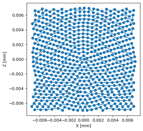
the range of positions strongly suggests, that the most likely unit is millimiters meaning the scan was covering an area of roughly \(14 x 14\) micrometers.
import matplotlib.pyplot as plt
plt.figure(figsize=(5,5))
plt.plot(posx,posz, marker="o")
plt.xlabel("X [mm]")
plt.ylabel("Z [mm]")
plt.show()
Plotting the diffraction patterns#
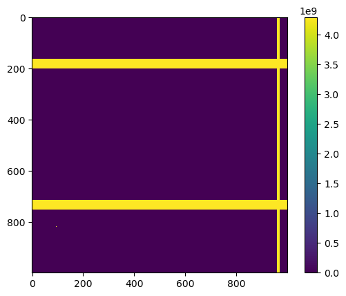
Next, we look at the diffraction data. Plotting the first image
import matplotlib.colors as colors
plt.figure()
plt.imshow(data[0], interpolation="none") # normal scale
#plt.imshow(data[0], interpolation="none", norm=colors.LogNorm()) # Log scale
plt.colorbar()
plt.show()
quickly reveals that there are some masked areas (invalid pixels) that need to be dealt with
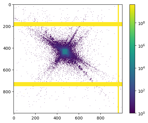
here is the same image but on a log scale
import matplotlib.colors as colors
plt.figure()
#plt.imshow(data[0], interpolation="none") # normal scale
plt.imshow(data[0], interpolation="none", norm=colors.LogNorm()) # Log scale
plt.colorbar()
plt.show()
Creating and saving a mask of invalid pixels#
To determine a mask of invalid pixels, it seems like we can simply threshold the first diffraction pattern
threshold = 4e9
mask = (data[0] > threshold)
fig, axes = plt.subplots(ncols=3, figsize=(10,3))
axes[0].set_title("Histogram of active pixels")
axes[0].hist(data[0][~mask].flatten(), bins=100)
axes[0].semilogy()
axes[1].set_title("Mask of inactive pixels")
axes[1].imshow(mask.astype(int), interpolation="none")
axes[2].set_title("Diffraction pattern")
axes[2].imshow(data[0] * (~mask), interpolation="none", norm=colors.LogNorm(vmin=0.1))
plt.show()
to obtain clean diffraction patterns with values between \(0\) and slightly above \(35,000\) counts
![]()
We finally save the mask in a new HDF5 file called eiger_mask.h5
with h5py.File("./eiger_mask.h5", "w") as f:
    f["data"] = mask.astype(int)
threshold = 4e9
mask = (data[0] > threshold)

fig, axes = plt.subplots(ncols=3, figsize=(10,3))
axes[0].set_title("Histogram of active pixels")
axes[0].hist(data[0][~mask].flatten(), bins=100)
axes[0].semilogy()
axes[1].set_title("Mask of inactive pixels")
axes[1].imshow(mask.astype(int), interpolation="none")
axes[2].set_title("Diffraction pattern")
axes[2].imshow(data[0] * (~mask), interpolation="none", norm=colors.LogNorm(vmin=0.1))
plt.show()

with h5py.File("./eiger_mask.h5", "w") as f:
    f["data"] = mask.astype(int)
Initial reconstruction steps#
There are other tutorials that already explain the different sections of the parameter tree, but it might be worth to go through them once again. After an initial part with imports
import ptypy, os
import ptypy.utils as u

# This will import the HDF5Loader class
ptypy.load_ptyscan_module("hdf5_loader")
we define how to obtain access to all relevant parts of the data file (path and keys)
# Path to the raw data
tutorial_data_home = "../../data/"
scan_nr = 32
#dataset = f"soleil_swing_siemens/nanoprobe3d_centrage_{scan_nr:05d}_2024-12-13_11-14-18.h5"
dataset = f"soleil_swing_siemens/nanoprobe3d_centrage_{scan_nr:05d}_2024-12-13_11-25-06.h5"
path_to_data = os.path.join(tutorial_data_home, dataset)
path_to_mask = "./eiger_mask.h5"

# Keys to data and metadata
root_entry = f"/SiemensStar_{scan_nr:05d}"
data_key = f"/{root_entry}/scan_data/eiger_image"
det_pixsize_key = f"/{root_entry}/SWING/EIGER-4M/pixel_size_x"
det_distance_key = f"/{root_entry}/SWING/EIGER-4M/distance"
sample_posx_key = f"/{root_entry}/scan_data/calc_gated_sample_tx"
sample_posz_key = f"/{root_entry}/scan_data/calc_gated_sample_tz"
photon_energy_key = f"/{root_entry}/SWING/i11-c-c03__op__mono/energy"
before starting to define the parameter tree, with the usual I/O settings for Jupyter notebooks and a frames_per_block of 100. This value could be increased, but given the scan has only \(632\) data points, \(100\) seems like a good compromise that should also work on GPUs with less memory.
# Create parameter tree
p = u.Param()

# Set verbose level to interactive
p.verbose_level = "interactive"

# Data blocks for loading
p.frames_per_block = 100

# Set io settings (no files saved)
p.io = u.Param()
p.io.rfile = None
p.io.autosave = u.Param(active=False)
p.io.interaction = u.Param(active=False)

# Live-plotting during the reconstruction
p.io.autoplot = u.Param()
p.io.autoplot.active=True
p.io.autoplot.threaded = False
p.io.autoplot.layout = "jupyter"
p.io.autoplot.interval = 10
Now, we need to define a “scan” and we choose the BlockFull model which is recommended for GPU reconstructions. We also need to provide an initial guess for the probe/illumination and this is one of the first more tricky parts. Probe retrieval is often the most difficult part of a ptychographic reconstruction and so defining a sensible initial guess can be very important for a successful reconstruction. The problem here is that we don’t know all that much about the properties of the illumination at the SWING beamline at specifically the experimental conditions for this particular data set. What we do know (by looking at the specs on their website) is that the beam is shaped by a KB system, which means we are expecting a rectangular aperture. At this point, the best thing would be to reach out to a beamline scientist and ask for the specifics, i.e. the size of the aperture (exit slit of the KB), the focal length (propagation.focussed) and how much the probe has been defocused during this experiment (propagation.parallel). But, let’s just carry on and see if we can figure it out by trial and error. Let’s assume a \(5x5\) mm aperture for now with a focal length of \(32\) m and \(3\) mm defocus
# Define the scan model
p.scans = u.Param()
p.scans.scan_00 = u.Param()
p.scans.scan_00.name = 'BlockFull'

# Initial illumination (based on simulated optics)
p.scans.scan_00.illumination = u.Param()
p.scans.scan_00.illumination.model = None
p.scans.scan_00.illumination.photons = None
p.scans.scan_00.illumination.aperture = u.Param()
p.scans.scan_00.illumination.aperture.form = "rect"
p.scans.scan_00.illumination.aperture.size = (5e-3,5e-3)
p.scans.scan_00.illumination.propagation = u.Param()
p.scans.scan_00.illumination.propagation.focussed = 32
p.scans.scan_00.illumination.propagation.parallel = 3e-3
Next, we need to tell PtyPy where to load the data from, for this we are going to use the HDF5Loader with the following settings
# Data loader
p.scans.scan_00.data = u.Param()
p.scans.scan_00.data.name = 'Hdf5Loader'
p.scans.scan_00.data.orientation = 0

# Read diffraction data
p.scans.scan_00.data.intensities = u.Param()
p.scans.scan_00.data.intensities.file = path_to_data
p.scans.scan_00.data.intensities.key = data_key

# Read positions data
p.scans.scan_00.data.positions = u.Param()
p.scans.scan_00.data.positions.file = path_to_data
p.scans.scan_00.data.positions.slow_key = sample_posx_key
p.scans.scan_00.data.positions.slow_multiplier = 1e-3
p.scans.scan_00.data.positions.fast_key = sample_posz_key
p.scans.scan_00.data.positions.fast_multiplier = 1e-3

# Read meta data: photon energy
p.scans.scan_00.data.recorded_energy = u.Param()
p.scans.scan_00.data.recorded_energy.file = path_to_data
p.scans.scan_00.data.recorded_energy.key = photon_energy_key
p.scans.scan_00.data.recorded_energy.multiplier = 1

# Read meta data: detector distance
p.scans.scan_00.data.recorded_distance = u.Param()
p.scans.scan_00.data.recorded_distance.file = path_to_data
p.scans.scan_00.data.recorded_distance.key = det_distance_key
p.scans.scan_00.data.recorded_distance.multiplier = 1e-3

# Read meta data: detector pixelsize
p.scans.scan_00.data.recorded_psize = u.Param()
p.scans.scan_00.data.recorded_psize.file = path_to_data
p.scans.scan_00.data.recorded_psize.key = det_pixsize_key
p.scans.scan_00.data.recorded_psize.multiplier = 1e-6

# Other metadata
p.scans.scan_00.data.shape = (512,512)
p.scans.scan_00.data.auto_center = True
Note, that we have set data.shape as \(512x512\) even the full size of the diffraction patterns is \(1000x1000\), this is to make the data loading and processing faster at the beginning - we can later increase the shape to obtain the highest possible resolution for the reconstruction. We have also turned on data.auto_center to automatically find the global centre of the diffraction patterns.
Finally, we can run PtyPy with ptypy.core.Ptycho() but we specify level=4 to stop just after the data is loaded, all the views and pods are created and the initial model for object and probe have been made.
# Run up until the creation of the initial model
P = ptypy.core.Ptycho(p,level=4)
import ptypy, os
import ptypy.utils as u

# This will import the HDF5Loader class
ptypy.load_ptyscan_module("hdf5_loader")

# Path to the raw data
tutorial_data_home = "../../data/"
scan_nr = 32
#dataset = f"soleil_swing_siemens/nanoprobe3d_centrage_{scan_nr:05d}_2024-12-13_11-14-18.h5"
dataset = f"soleil_swing_siemens/nanoprobe3d_centrage_{scan_nr:05d}_2024-12-13_11-25-06.h5"
path_to_data = os.path.join(tutorial_data_home, dataset)
path_to_mask = "./eiger_mask.h5"

# Keys to data and metadata
root_entry = f"/SiemensStar_{scan_nr:05d}"
data_key = f"/{root_entry}/scan_data/eiger_image"
det_pixsize_key = f"/{root_entry}/SWING/EIGER-4M/pixel_size_x"
det_distance_key = f"/{root_entry}/SWING/EIGER-4M/distance"
sample_posx_key = f"/{root_entry}/scan_data/calc_gated_sample_tx"
sample_posz_key = f"/{root_entry}/scan_data/calc_gated_sample_tz"
photon_energy_key = f"/{root_entry}/SWING/i11-c-c03__op__mono/energy"

# Create parameter tree
p = u.Param()

# Set verbose level to interactive
p.verbose_level = "interactive"

# Data blocks for loading
p.frames_per_block = 100

# Set io settings (no files saved)
p.io = u.Param()
p.io.rfile = None
p.io.autosave = u.Param(active=False)
p.io.interaction = u.Param(active=False)

# Live-plotting during the reconstruction
p.io.autoplot = u.Param()
p.io.autoplot.active=True
p.io.autoplot.threaded = False
p.io.autoplot.layout = "jupyter"
p.io.autoplot.interval = 10

# Define the scan model
p.scans = u.Param()
p.scans.scan_00 = u.Param()
p.scans.scan_00.name = 'BlockFull'

# Initial illumination (based on simulated optics)
p.scans.scan_00.illumination = u.Param()
p.scans.scan_00.illumination.model = None
p.scans.scan_00.illumination.photons = None
p.scans.scan_00.illumination.aperture = u.Param()
p.scans.scan_00.illumination.aperture.form = "rect"
p.scans.scan_00.illumination.aperture.size = (5e-3,5e-3)
p.scans.scan_00.illumination.propagation = u.Param()
p.scans.scan_00.illumination.propagation.focussed = 32
p.scans.scan_00.illumination.propagation.parallel = 3e-3

# Data loader
p.scans.scan_00.data = u.Param()
p.scans.scan_00.data.name = 'Hdf5Loader'
p.scans.scan_00.data.orientation = 0

# Read diffraction data
p.scans.scan_00.data.intensities = u.Param()
p.scans.scan_00.data.intensities.file = path_to_data
p.scans.scan_00.data.intensities.key = data_key

# Read positions data
p.scans.scan_00.data.positions = u.Param()
p.scans.scan_00.data.positions.file = path_to_data
p.scans.scan_00.data.positions.slow_key = sample_posx_key
p.scans.scan_00.data.positions.slow_multiplier = 1e-3
p.scans.scan_00.data.positions.fast_key = sample_posz_key
p.scans.scan_00.data.positions.fast_multiplier = 1e-3

# Load mask from file
p.scans.scan_00.data.mask = u.Param()
p.scans.scan_00.data.mask.file = path_to_mask
p.scans.scan_00.data.mask.key = "data"
p.scans.scan_00.data.mask.invert = True

# Read meta data: photon energy
p.scans.scan_00.data.recorded_energy = u.Param()
p.scans.scan_00.data.recorded_energy.file = path_to_data
p.scans.scan_00.data.recorded_energy.key = photon_energy_key
p.scans.scan_00.data.recorded_energy.multiplier = 1

# Read meta data: detector distance
p.scans.scan_00.data.recorded_distance = u.Param()
p.scans.scan_00.data.recorded_distance.file = path_to_data
p.scans.scan_00.data.recorded_distance.key = det_distance_key
p.scans.scan_00.data.recorded_distance.multiplier = 1e-3

# Read meta data: detector pixelsize
p.scans.scan_00.data.recorded_psize = u.Param()
p.scans.scan_00.data.recorded_psize.file = path_to_data
p.scans.scan_00.data.recorded_psize.key = det_pixsize_key
p.scans.scan_00.data.recorded_psize.multiplier = 1e-6

# Other metadata
p.scans.scan_00.data.shape = (512,512)
p.scans.scan_00.data.auto_center = True

# Run reconstruction
P = ptypy.core.Ptycho(p,level=4)
Optimising the initial probe#
In order to inspect the initial probe calculated by PtyPy, the easiest way is to take the first pod and look at pod.probe. We can also us the forward projector pod.fw() to calculate how our initial probe looks like in Fourier space and compare it to the diffraction data
pod = list(P.pods.values())[0]
probe = pod.probe
Fprobe = u.abs2(pod.fw(pod.probe))
the following code will plot those images side by side
fig, axes = plt.subplots(ncols=3, figsize=(15,5), dpi=100)
ax0 = u.PtyAxis(axes[0], channel="c")
ax0.set_data(probe)
axes[1].imshow(Fprobe)
axes[2].imshow(data[0,180:180+512,230:230+512])
plt.show()
looking like this
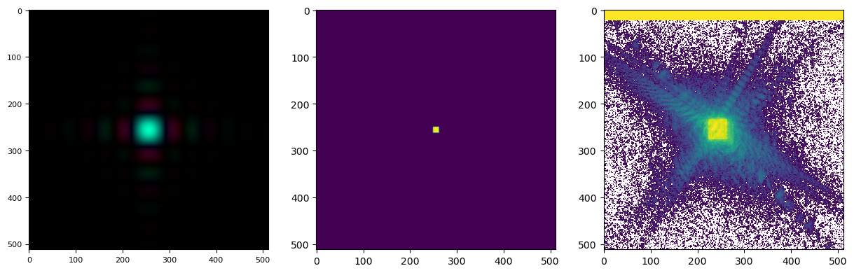
showing that our probe in the diffraction plane is too small. With a bit of trial and error, we can arrive at a reasonable initial probe at an aperture size of \(15x15\) mm, the same initial focal length of \(32\) m and a defocus of \(5\) mm to make sure the probe is filling the space nicely. Note that it does not matter that those optical properties could all be wrong, what matters is that we arrived at a reasonably shaped intial probe both in real and Fourier space. The final result looks like this
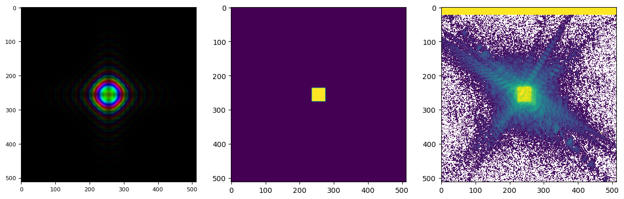
pod = list(P.pods.values())[0]
probe = pod.probe
Fprobe = u.abs2(pod.fw(pod.probe))
fig, axes = plt.subplots(ncols=3, figsize=(15,5), dpi=100)
ax0 = u.PtyAxis(axes[0], channel="c")
ax0.set_data(probe)
axes[1].imshow(Fprobe)
axes[2].imshow(data[0,180:180+512,230:230+512], norm=colors.LogNorm(vmin=0.1, vmax=3e4))
plt.show()
Let’s give the reconstruction a go#
We can largerly use the same parameter as outlined above, with a few changes. First, we need to load the cupy engines
# This will import the GPU engines
ptypy.load_gpu_engines("cupy")
we also need to load the mask of invalid pixels that we have generated earlier, note that you might need to use the mask.invert parameter to invert that masked values. By default the HDf5Loader is considering the valid pixels as masked (1 in the mask) and the invalid pixels as non-masked (0 in the mask).
# Load mask from file
p.scans.scan_00.data.mask = u.Param()
p.scans.scan_00.data.mask.file = path_to_mask
p.scans.scan_00.data.mask.key = "data"
p.scans.scan_00.data.mask.invert = True
and finally, we need to add a reconstruction - here we use difference map with mostly standard parameters but a few tweaks
# Define reconstruction engine (using DM)
p.engines = u.Param()
p.engines.engine = u.Param()
p.engines.engine.name = "DM_cupy"
p.engines.engine.numiter = 100
p.engines.engine.numiter_contiguous = 5
p.engines.engine.alpha = 0.9
p.engines.engine.probe_support = None
p.engines.engine.probe_update_start = 0
making sure that we start updating the probe from the very beginning (engine.probe_update_start = 0, set alpha to \(0.9\) - this makes the difference map update a bit less agressive and is usually advantageous when working with real data. We set the nr. of iterations to \(100\) which is typically enough to judge whether a reconstruction is going in the right direction or if something is wrong.
We can now start our first attempt and reconstructing the data
# Run reconstruction
P = ptypy.core.Ptycho(p,level=5)
and the result is…
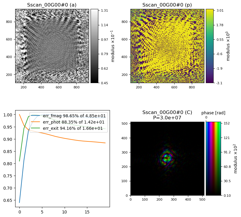
hmm, that does not look right. We need to make some changes…
import ptypy, os
import ptypy.utils as u

# This will import the HDF5Loader class
ptypy.load_ptyscan_module("hdf5_loader")

# This will import the GPU engines
ptypy.load_gpu_engines("cupy")

# Path to the raw data
tutorial_data_home = "../../data/"
scan_nr = 32
#dataset = f"soleil_swing_siemens/nanoprobe3d_centrage_{scan_nr:05d}_2024-12-13_11-14-18.h5"
dataset = f"soleil_swing_siemens/nanoprobe3d_centrage_{scan_nr:05d}_2024-12-13_11-25-06.h5"
path_to_data = os.path.join(tutorial_data_home, dataset)
path_to_mask = "./eiger_mask.h5"

# Keys to data and metadata
root_entry = f"/SiemensStar_{scan_nr:05d}"
data_key = f"/{root_entry}/scan_data/eiger_image"
det_pixsize_key = f"/{root_entry}/SWING/EIGER-4M/pixel_size_x"
det_distance_key = f"/{root_entry}/SWING/EIGER-4M/distance"
sample_posx_key = f"/{root_entry}/scan_data/calc_gated_sample_tx"
sample_posz_key = f"/{root_entry}/scan_data/calc_gated_sample_tz"
photon_energy_key = f"/{root_entry}/SWING/i11-c-c03__op__mono/energy"

# Create parameter tree
p = u.Param()

# Set verbose level to interactive
p.verbose_level = "interactive"

# Data blocks for loading
p.frames_per_block = 100

# Set io settings (no files saved)
p.io = u.Param()
p.io.rfile = None
p.io.autosave = u.Param(active=False)
p.io.interaction = u.Param(active=False)

# Live-plotting during the reconstruction
p.io.autoplot = u.Param()
p.io.autoplot.active=True
p.io.autoplot.threaded = False
p.io.autoplot.layout = "jupyter"
p.io.autoplot.interval = 10

# Define the scan model
p.scans = u.Param()
p.scans.scan_00 = u.Param()
p.scans.scan_00.name = 'BlockFull'

# Initial illumination (based on simulated optics)
p.scans.scan_00.illumination = u.Param()
p.scans.scan_00.illumination.model = None
p.scans.scan_00.illumination.photons = None
p.scans.scan_00.illumination.aperture = u.Param()
p.scans.scan_00.illumination.aperture.form = "rect"
p.scans.scan_00.illumination.aperture.size = (15e-3,15e-3)
p.scans.scan_00.illumination.propagation = u.Param()
p.scans.scan_00.illumination.propagation.focussed = 32
p.scans.scan_00.illumination.propagation.parallel = 5e-3

# Data loader
p.scans.scan_00.data = u.Param()
p.scans.scan_00.data.name = 'Hdf5Loader'
p.scans.scan_00.data.orientation = 6

# Read diffraction data
p.scans.scan_00.data.intensities = u.Param()
p.scans.scan_00.data.intensities.file = path_to_data
p.scans.scan_00.data.intensities.key = data_key

# Read positions data
p.scans.scan_00.data.positions = u.Param()
p.scans.scan_00.data.positions.file = path_to_data
p.scans.scan_00.data.positions.slow_key = sample_posx_key
p.scans.scan_00.data.positions.slow_multiplier = 1e-3
p.scans.scan_00.data.positions.fast_key = sample_posz_key
p.scans.scan_00.data.positions.fast_multiplier = 1e-3

# Load mask from file
p.scans.scan_00.data.mask = u.Param()
p.scans.scan_00.data.mask.file = path_to_mask
p.scans.scan_00.data.mask.key = "data"
p.scans.scan_00.data.mask.invert = True

# Read meta data: photon energy
p.scans.scan_00.data.recorded_energy = u.Param()
p.scans.scan_00.data.recorded_energy.file = path_to_data
p.scans.scan_00.data.recorded_energy.key = photon_energy_key
p.scans.scan_00.data.recorded_energy.multiplier = 1

# Read meta data: detector distance
p.scans.scan_00.data.recorded_distance = u.Param()
p.scans.scan_00.data.recorded_distance.file = path_to_data
p.scans.scan_00.data.recorded_distance.key = det_distance_key
p.scans.scan_00.data.recorded_distance.multiplier = 1e-3

# Read meta data: detector pixelsize
p.scans.scan_00.data.recorded_psize = u.Param()
p.scans.scan_00.data.recorded_psize.file = path_to_data
p.scans.scan_00.data.recorded_psize.key = det_pixsize_key
p.scans.scan_00.data.recorded_psize.multiplier = 1e-6

# Load mask from file
p.scans.scan_00.data.mask = u.Param()
p.scans.scan_00.data.mask.file = path_to_mask
p.scans.scan_00.data.mask.key = "data"
p.scans.scan_00.data.mask.invert = True

# Other metadata
p.scans.scan_00.data.shape = (512,512)
p.scans.scan_00.data.auto_center = True

p.engines = u.Param()
p.engines.engine = u.Param()
p.engines.engine.name = "DM_cupy"
p.engines.engine.numiter = 100
p.engines.engine.numiter_contiguous = 5
p.engines.engine.alpha = 0.9
p.engines.engine.probe_support = None
p.engines.engine.probe_update_start = 0

# Run reconstruction
P = ptypy.core.Ptycho(p,level=5)
Let’s make it work#
We have now arrived at arguably the most difficult part of our task to reconstruct new data from scratch. We think that we have provided all the correct data or at least some reasonable estimates, but the reconstruction still looks completely wrong. At this point, it is advised to carefully check that all the provided numbers have the correct units, i.e. photon energy, detector distance, detector pixel size, the scan positions and they are indeed correct. If we are using a mask, we should also double check that it is loaded correctly or if it needs to be inverted. Once we have double checked all of this, there is one last barrier to overcome: choosing the correct coordinate system.
Unfortunately, there is no guarantee that the coordinate system chosen and implemented by the PtyPy developers (right-handed with the X-axis pointing with the beam) and the local coordinate system used at the beamline together with how we have loaded in that data/posisitions (i.e. positions.slow_key vs. positions.fast_key) are actual matching precisely. It is actually quite likely that there is a mismatch. Here we could again reach out to the beamline scientist and figure out how the data has been collected and saved, but in most cases it might be faster to simply try all permutations. Fortunately, there are only 8 possible combinations and PtyPy has a convenient parameter data.orientation that allows us to quickly try all of these combinations - the default value is \(0\). For a full description of the possible combinations and what they are, have a look at the definition here
# Data loader
p.scans.scan_00.data = u.Param()
p.scans.scan_00.data.name = 'Hdf5Loader'
p.scans.scan_00.data.orientation = 0
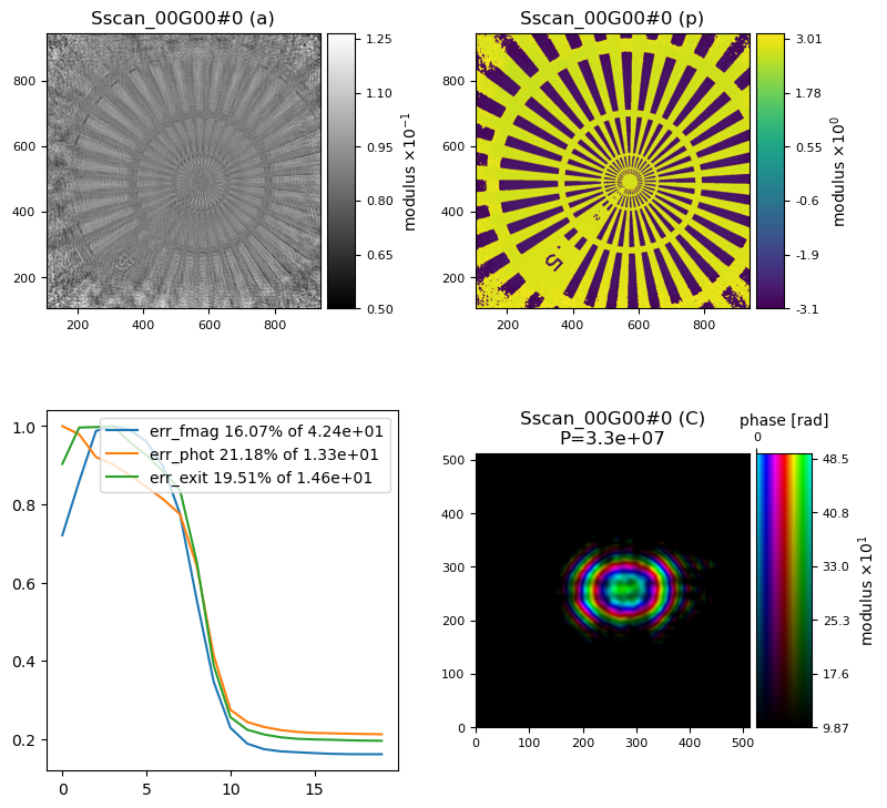
Challenge
Change the orientation parameter until you are satisfied with the result.
Once you find the correct orientation, i.e. a match between PtyPy’s coordinate system and the way how this dataset has been collected and loaded, the final result should look like this