Maximum Likelihood with the wavefield pre-conditioner#
Learning how to use the maximum-likelihood engine with the wavefield preconditioner and it comparing the results with other more explorative engines like difference map
Inspired by this paper on iterative least-squares solvers for ptychography - specifically equations (25a) and (25b), we have recently implemented a wavefield preconditioner for the maximum-likelihood engine (available as of Release 0.9). The idea behind this is that by rescaling both the updates for the object and probes by a “fluence” field, the optimisation happens in the more natural wavefield space and therefore accelerates the convergence of ML, especially when the initial estimates of probe and object are further away from the solution - a common problem with the regular ML engine. In this tutorial, we are exploring this new feature based on the data from the SOLEIL/SWING tutorial. As a bonus, this tutorial also illustrates how a given state (i.e. before running any engine or after a particular engine is finished) can be saved and restored.
Making sure there is a mask file#
import h5py, os
import numpy as np

tutorial_data_home = "../../data/"
scan_nr = 32
#dataset = f"soleil_swing_siemens/nanoprobe3d_centrage_{scan_nr:05d}_2024-12-13_11-14-18.h5"
dataset = f"soleil_swing_siemens/nanoprobe3d_centrage_{scan_nr:05d}_2024-12-13_11-25-06.h5"
path_to_data = os.path.join(tutorial_data_home, dataset)

root_entry = f"/SiemensStar_{scan_nr:05d}"
data_key = f"/{root_entry}/scan_data/eiger_image"

with h5py.File(path_to_data, "r") as f:
    data = f[data_key][0]

threshold = 4e9
mask = (data > threshold)
with h5py.File("./eiger_mask.h5", "w") as f:
    f["data"] = mask.astype(int)
Regualar approach: DM + ML#
A quite common approach is to first us the more explorative difference map (DM) algorithm followed by a few iterations of the maximum-likelihood algorithm. In PtyPy, this is quite easy to achieve by simply chaining the engines in the parameter tree
# Define reconstruction engine (using DM)
p.engines = u.Param()
p.engines.engine1 = u.Param()
p.engines.engine1.name = "DM_cupy"
p.engines.engine1.numiter = 150
p.engines.engine1.numiter_contiguous = 5
p.engines.engine1.alpha = 0.9
p.engines.engine1.probe_support = None
p.engines.engine1.probe_update_start = 0
p.engines.engine1.fft_lib = "cuda"
p.engines.engine1.overlap_converge_factor = 0.001
p.engines.engine1.update_object_first = True
p.engines.engine1.obj_smooth_std = 20
p.engines.engine1.probe_inertia = 0.001
p.engines.engine1.object_inertia = 0.001
p.engines.engine1.fourier_power_bound = 0.0
p.engines.engine1.record_local_error = False

p.engines.engine2 = u.Param()
p.engines.engine2.name = "ML_cupy"
p.engines.engine2.numiter = 50
p.engines.engine2.numiter_contiguous = 5
p.engines.engine2.reg_del2 = False
p.engines.engine2.reg_del2_amplitude = 0.01
p.engines.engine2.scale_precond = False
p.engines.engine2.probe_support = None
p.engines.engine2.probe_update_start = 0
p.engines.engine2.fft_lib = "cuda"
Note that compare to the basic tutorial, we are now using as close as possible to the original size of the diffraction data by setting
p.scans.scan_00.data.shape = (950,950)
and in order to only load the data into memory once, we can save the initial state of the reconstruction (before any engine is executed) like so
# Load, prepare and save state
P = ptypy.core.Ptycho(p,level=4)
P.copy_state("initial")
before running the DM + ML engines
P.run(epars=p.engines.engine1)
P.run(epars=p.engines.engine2)
P.copy_state("DM + regular ML")
import ptypy, os
import ptypy.utils as u

# This will import the HDF5Loader class
ptypy.load_ptyscan_module("hdf5_loader")

# This will import the GPU engines
ptypy.load_gpu_engines("cupy")

# Path to the raw data
tutorial_data_home = "../../data/"
scan_nr = 32
#dataset = f"soleil_swing_siemens/nanoprobe3d_centrage_{scan_nr:05d}_2024-12-13_11-14-18.h5"
dataset = f"soleil_swing_siemens/nanoprobe3d_centrage_{scan_nr:05d}_2024-12-13_11-25-06.h5"
path_to_data = os.path.join(tutorial_data_home, dataset)
path_to_mask = "./eiger_mask.h5"

# Keys to data and metadata
root_entry = f"/SiemensStar_{scan_nr:05d}"
data_key = f"/{root_entry}/scan_data/eiger_image"
det_pixsize_key = f"/{root_entry}/SWING/EIGER-4M/pixel_size_x"
det_distance_key = f"/{root_entry}/SWING/EIGER-4M/distance"
sample_posx_key = f"/{root_entry}/scan_data/calc_gated_sample_tx"
sample_posz_key = f"/{root_entry}/scan_data/calc_gated_sample_tz"
photon_energy_key = f"/{root_entry}/SWING/i11-c-c03__op__mono/energy"

# Create parameter tree
p = u.Param()

# Set verbose level to interactive
p.verbose_level = "interactive"

# Data blocks for loading
p.frames_per_block = 100

# Set io settings (no files saved)
p.io = u.Param()
p.io.rfile = None
p.io.autosave = u.Param(active=False)
p.io.interaction = u.Param(active=False)

# Live-plotting during the reconstruction
p.io.autoplot = u.Param()
p.io.autoplot.active=True
p.io.autoplot.threaded = False
p.io.autoplot.layout = "jupyter"
p.io.autoplot.interval = 5

# Define the scan model
p.scans = u.Param()
p.scans.scan_00 = u.Param()
p.scans.scan_00.name = 'BlockFull'

# Initial illumination (based on simulated optics)
p.scans.scan_00.illumination = u.Param()
p.scans.scan_00.illumination.model = None
p.scans.scan_00.illumination.photons = None
p.scans.scan_00.illumination.aperture = u.Param()
p.scans.scan_00.illumination.aperture.form = "rect"
p.scans.scan_00.illumination.aperture.size = (15e-3,15e-3)
p.scans.scan_00.illumination.propagation = u.Param()
p.scans.scan_00.illumination.propagation.focussed = 32
p.scans.scan_00.illumination.propagation.parallel = 6e-3

# Data loader
p.scans.scan_00.data = u.Param()
p.scans.scan_00.data.name = 'Hdf5Loader'
p.scans.scan_00.data.orientation = 6

# Read diffraction data
p.scans.scan_00.data.intensities = u.Param()
p.scans.scan_00.data.intensities.file = path_to_data
p.scans.scan_00.data.intensities.key = data_key

# Read positions data
p.scans.scan_00.data.positions = u.Param()
p.scans.scan_00.data.positions.file = path_to_data
p.scans.scan_00.data.positions.slow_key = sample_posx_key
p.scans.scan_00.data.positions.slow_multiplier = 1e-3
p.scans.scan_00.data.positions.fast_key = sample_posz_key
p.scans.scan_00.data.positions.fast_multiplier = 1e-3

# Load mask from file
p.scans.scan_00.data.mask = u.Param()
p.scans.scan_00.data.mask.file = path_to_mask
p.scans.scan_00.data.mask.key = "data"
p.scans.scan_00.data.mask.invert = True

# Read meta data: photon energy
p.scans.scan_00.data.recorded_energy = u.Param()
p.scans.scan_00.data.recorded_energy.file = path_to_data
p.scans.scan_00.data.recorded_energy.key = photon_energy_key
p.scans.scan_00.data.recorded_energy.multiplier = 1

# Read meta data: detector distance
p.scans.scan_00.data.recorded_distance = u.Param()
p.scans.scan_00.data.recorded_distance.file = path_to_data
p.scans.scan_00.data.recorded_distance.key = det_distance_key
p.scans.scan_00.data.recorded_distance.multiplier = 1e-3

# Read meta data: detector pixelsize
p.scans.scan_00.data.recorded_psize = u.Param()
p.scans.scan_00.data.recorded_psize.file = path_to_data
p.scans.scan_00.data.recorded_psize.key = det_pixsize_key
p.scans.scan_00.data.recorded_psize.multiplier = 1e-6

# Other metadata
p.scans.scan_00.data.shape = (950,950)
p.scans.scan_00.data.auto_center = True

# Define reconstruction engine (using DM)
p.engines = u.Param()
p.engines.engine1 = u.Param()
p.engines.engine1.name = "DM_cupy"
p.engines.engine1.numiter = 150
p.engines.engine1.numiter_contiguous = 5
p.engines.engine1.alpha = 0.9
p.engines.engine1.probe_support = None
p.engines.engine1.probe_update_start = 0
p.engines.engine1.fft_lib = "cuda"
p.engines.engine1.overlap_converge_factor = 0.001
p.engines.engine1.update_object_first = True
p.engines.engine1.obj_smooth_std = 20
p.engines.engine1.probe_inertia = 0.001
p.engines.engine1.object_inertia = 0.001
p.engines.engine1.fourier_power_bound = 0.0
p.engines.engine1.record_local_error = False

p.engines.engine2 = u.Param()
p.engines.engine2.name = "ML_cupy"
p.engines.engine2.numiter = 50
p.engines.engine2.numiter_contiguous = 5
p.engines.engine2.reg_del2 = False
p.engines.engine2.reg_del2_amplitude = 0.01
p.engines.engine2.scale_precond = False
p.engines.engine2.probe_support = None
p.engines.engine2.probe_update_start = 0
p.engines.engine2.fft_lib = "cuda"

# Load, prepare and save state
P = ptypy.core.Ptycho(p,level=4)
P.copy_state("initial")
P.run(epars=p.engines.engine1)
P.run(epars=p.engines.engine2)
P.copy_state("DM + regular ML")
New approach: ML with wavefield preconditioner#
We can now add another ML engine to the parameter tree with the wavefield_precond featured enabled
# Define reconstruction engine using only ML
p.engines.engine3 = u.Param()
p.engines.engine3.name = "ML_cupy"
p.engines.engine3.numiter = 500
p.engines.engine3.numiter_contiguous = 5
p.engines.engine3.reg_del2 = False
p.engines.engine3.reg_del2_amplitude = 0.01
p.engines.engine3.scale_precond = False
p.engines.engine3.probe_support = None
p.engines.engine3.probe_update_start = 0
p.engines.engine3.wavefield_precond = True
and before running this engine, we restore the initial state that have saved earlier making sure that we are starting again from the initial probe and object
P.restore_state(name="initial")
P.run(epars=p.engines.engine3)
P.copy_state("ML with wavefield precond")
P.finalize()
# Define reconstruction engine using only ML
p.engines.engine3 = u.Param()
p.engines.engine3.name = "ML_cupy"
p.engines.engine3.numiter = 500
p.engines.engine3.numiter_contiguous = 5
p.engines.engine3.reg_del2 = False
p.engines.engine3.reg_del2_amplitude = 0.01
p.engines.engine3.scale_precond = False
p.engines.engine3.probe_support = None
p.engines.engine3.probe_update_start = 0
p.engines.engine3.wavefield_precond = True
P.restore_state(name="initial")
P.run(epars=p.engines.engine3)
P.copy_state("ML with wavefield precond")
P.finalize()
Comparing the results#
It is now time to compare the results, we can access the reconstructed objects from the states we have saved earlier by directly accessing P.state_dict
obj_dm_ml = P.state_dict["DM + regular ML"]["ob"].storages["Sscan_00G00"].data[0]
obj_ml_wf = P.state_dict["ML with wavefield precond"]["ob"].storages["Sscan_00G00"].data[0]
and after normalising the reconstructions to have median-zero phase
obj_dm_ml *= np.exp(-1j*np.median(np.angle(obj_dm_ml)))
obj_ml_wf *= np.exp(-1j*np.median(np.angle(obj_ml_wf)))
we can plot the results
import numpy as np
import matplotlib.pyplot as plt
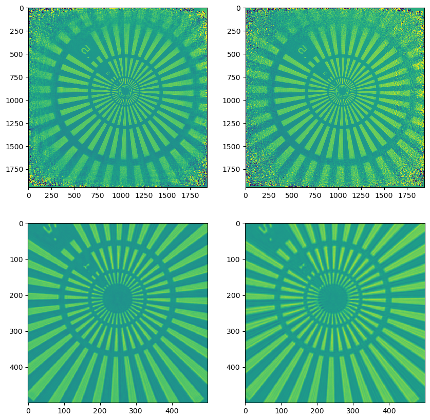
fig, axes = plt.subplots(ncols=2, nrows=2, figsize=(10,10))
axes[0,0].imshow(np.angle(obj_dm_ml), interpolation="none", cmap="viridis", vmin=-0.5*np.pi, vmax=0.5*np.pi)
axes[0,1].imshow(np.angle(obj_ml_wf), interpolation="none", cmap="viridis", vmin=-0.5*np.pi, vmax=0.5*np.pi)
axes[1,0].imshow(np.angle(obj_dm_ml)[700:1200,800:1300], interpolation="none", cmap="viridis", vmin=-0.5*np.pi, vmax=0.5*np.pi)
axes[1,1].imshow(np.angle(obj_ml_wf)[700:1200,800:1300], interpolation="none", cmap="viridis", vmin=-0.5*np.pi, vmax=0.5*np.pi)
plt.show()
showing as that indeed, ML with the wavefield pre-conditioner is capable of producing similar results compared to the regular approach of DM+ML
obj_dm_ml = P.state_dict["DM + regular ML"]["ob"].storages["Sscan_00G00"].data[0]
obj_ml_wf = P.state_dict["ML with wavefield precond"]["ob"].storages["Sscan_00G00"].data[0]
obj_dm_ml *= np.exp(-1j*np.median(np.angle(obj_dm_ml)))
obj_ml_wf *= np.exp(-1j*np.median(np.angle(obj_ml_wf)))
import numpy as np
import matplotlib.pyplot as plt
fig, axes = plt.subplots(ncols=2, nrows=2, figsize=(10,10))
axes[0,0].imshow(np.angle(obj_dm_ml), interpolation="none", cmap="viridis", vmin=-0.5*np.pi, vmax=0.5*np.pi)
axes[0,1].imshow(np.angle(obj_ml_wf), interpolation="none", cmap="viridis", vmin=-0.5*np.pi, vmax=0.5*np.pi)
axes[1,0].imshow(np.angle(obj_dm_ml)[700:1200,800:1300], interpolation="none", cmap="viridis", vmin=-0.5*np.pi, vmax=0.5*np.pi)
axes[1,1].imshow(np.angle(obj_ml_wf)[700:1200,800:1300], interpolation="none", cmap="viridis", vmin=-0.5*np.pi, vmax=0.5*np.pi)
plt.savefig("./_assets/soleil_swing_ml_wavefield_comparison.png", dpi=100, bbox_inches="tight")
plt.show()